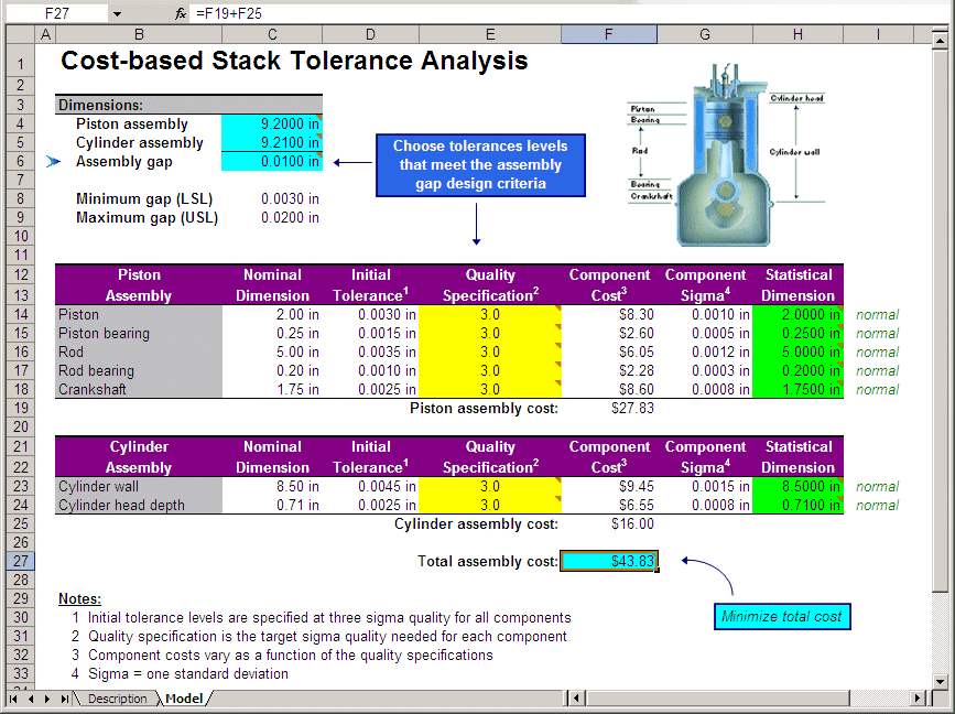
Open the Tolerance Analysis.xls file (Figure 52, Tolerance analysis spreadsheet model).
A drawing of the assembly is in the corner. In this example:
Initial tolerances of each 3-sigma component are in cells D14:D18 and D23:D24.
The relationship between the initial tolerance and the quality specifications (cells E14:E18 and E23:E24) yields a component sigma (cells G14:G18 and G23:G24).
The statistical dimension (cells H14:H18 and H23:H24) of each component is defined as an assumption with a normal distribution having a mean equal to the nominal dimension and a standard deviation equal to the component sigma. Note that the mean and standard deviation are cell references to these cells.
The dimensions of the assemblies are a cumulation of their respective components’ statistical dimensions. The difference in length between the cylinder assembly (cell C5) and the piston assembly (cell C4) is the assembly gap (cell C6).
Component cost (cells F14:F18 and F23:F24) is a nonlinear function of quality specification. The higher the specification, the higher the cost. Also note that each component has a different cost function associated with it.
In addition to the recommended options, before running OptQuest, in Crystal Ball select Run, Run Preferences and set:
On the Statistics tab of the Run Preferences dialog, select Calculate capability metrics.
Since the model is heavily dependent on the tails of the forecast distribution, these settings will provide higher accuracy and will be adequate for this example. In actual practice, to gain better accuracy, the engineer might want to run longer simulations of 5000 or 10,000 trials.
