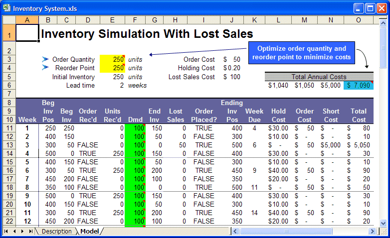
Before examining the spreadsheet simulation model, step through the logic of how this inventory system operates. Assume that no orders are outstanding initially and that the initial inventory level is equal to the order quantity, Q. Therefore, the beginning inventory position will be the same as the inventory level. At the beginning of the week, if any outstanding orders have arrived, the manager adds the order quantity to the current inventory level.
Next, determine the weekly demand and check if sufficient inventory is on hand to meet this demand. If not, then the number of lost sales is the demand minus the current inventory. Subtract the current inventory level from the inventory position, set current inventory to zero, and compute the lost sales cost. If sufficient inventory is available, satisfy all demand from stock and reduce both the inventory level and inventory position by the amount of demand.
The next step is to check if the inventory position is at or below the reorder point. If so, place an order for Q units and compute the order cost. The inventory position is increased by Q, but the inventory level remains the same. Schedule a receipt of Q units to arrive after the lead-time.
Finally, compute the holding cost based on the inventory level at the end of the week (after demand is satisfied) and the total cost.
Open the file Inventory System.xls. This spreadsheet model, shown in Figure 54, Inventory system problem spreadsheet model, implements this logic.The basic problem data are shown several rows down from the title. The decision variables are the order quantity (cell E3) and the reorder point (cell E4). The initial inventory is set equal to the chosen order quantity. This example assumes the specified lead-time is constant.
In the actual simulation, the beginning inventory position and inventory level for each week equals the ending levels for the previous week, except for the first week, which is specified in the problem data. The demand is in column F as Crystal Ball assumptions.
Since all shortages are lost sales, the inventory level cannot be negative. Thus, the ending inventory each week is:
Lost sales are computed by checking if demand exceeds available stock and computing the difference.
The spreadsheet simulates 52 weeks, or one year of operation of the inventory system. Since the objective is to minimize the mean total annual cost, cell O6 is defined as a forecast cell.
Column I determines whether the manager should place an order by checking if the beginning inventory position minus the weekly demand is at or below the reorder point. The ending inventory position is:
This formula might not appear to be obvious. Clearly, if there are no lost sales, the ending inventory position is simply the beginning position minus the demand plus any order that may have been placed. If lost sales occur, computing the ending inventory position this way reduces it by the unfulfilled demand, which is incorrect. Thus, you must add back the number of lost sales to account for this.
In the ordering process, the manager places orders at the end of the week and receives orders at the beginning of the week. Thus, in Figure 54, Inventory system problem spreadsheet model, the order placed at the end of the first week with a lead-time of 2 weeks will arrive at the beginning of the fourth week. Column K determines the week an order is due to arrive, and a MATCH function is used in column D to identify whether an order is scheduled to arrive.


