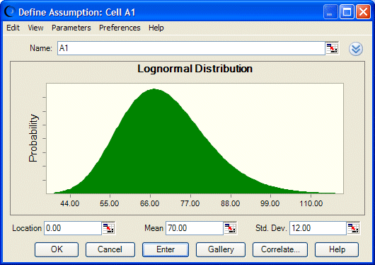
The lognormal distribution can be used to model the price of a particular stock. You purchase a stock today at $50. You expect that the stock will be worth $70 at the end of the year. If the stock price drops at the end of the year, rather than appreciating, you know that the lowest value it can drop to is $0.
On the other hand, the stock could end up with a price much higher than expected, thus implying no upper limit on the rate of return. In summary, the losses are limited to the original investment, but the gains are unlimited.
Using historical data, you can determine that the standard deviation of the stock’s price is $12.
If you have historical data available with which to define a lognormal distribution, it is important to calculate the mean and standard deviation of the logarithms of the data and then enter these log parameters using the Parameters menu (Location, Log Mean, and Log Standard Deviation). Calculating the mean and standard deviation directly on the raw data will not give you the correct lognormal distribution. Alternatively, use the distribution fitting feature described in Fitting Distributions to Data. |
The first step in selecting a probability distribution is matching the data with a distribution’s conditions. Checking the lognormal distribution:
These conditions match those of the lognormal distribution (Figure 103, Lognormal distribution).
In the lognormal distribution, the mean parameter is set at $70.00 and the standard deviation set at $12.00. The default location is 0, which works for this example. This distribution shows the probability that the stock price will be $x.
