Vision Research has determined that nearsightedness afflicts nearly 40 million people in the United States, and an additional 0% to 5% of these people will develop this condition during the year in which ClearView is tested.
However, the marketing department has learned that a 25% chance exists that a competing product will be released on the market soon. This product would decrease ClearView’s potential market by 5% to 15%.
Since the uncertainties in this situation require a unique approach, Vision Research selects Crystal Ball’s custom distribution to define the growth rate.
The method for specifying parameters in the custom distribution is quite unlike the other distribution types, so follow the directions carefully. If you make a mistake, click Gallery to return to the distribution gallery, then start again at step 4.
Use the custom distribution to plot both the potential increase and decrease of ClearView’s market.
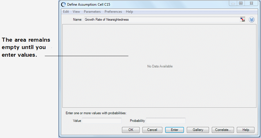
 To define the assumption cell for the growth rate of nearsightedness:
Click All in the navigation pane of the Distribution Gallery to show all distributions shipped with Crystal Ball.
Scroll down to the end of the Distribution Gallery and click the Custom distribution.
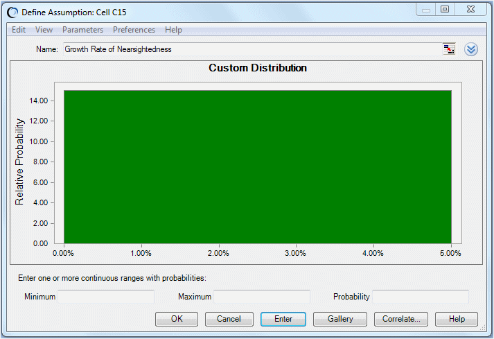
The Custom Distribution dialog opens.
Notice in Figure 117, Custom Distribution Dialog that the chart area remains empty until you specify the Parameters type and enter the values for the distribution.
You know that you will be working with two distribution ranges: one showing growth in nearsightedness and one showing the effects of competition. Both ranges are continuous.
Select Continuous Ranges in the Parameters menu.
The Custom Distribution dialog now has three parameters: Minimum, Maximum, and Probability.
Enter the first range of values to show the growth of nearsightedness with low probability of competitive effects:
Type 75% or .75 in the Probability text box.
This represents the 75% chance that Vision Research’s competitor will not enter the market and reduce Vision Research’s share.
A uniform distribution for the first range of values, 0% to 5%, is displayed (Figure 118, Uniform Distribution Range.
Notice that the total area of the range is equal to the probability: 5% wide by 15 units high equals 75%.
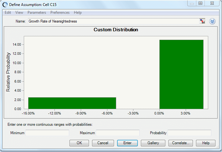
Now, enter a second range of values to show the effect of competition:
Type 25% in the Probability text box.
This represents the 25% chance that Vision Research’s competitor will enter the market place and decrease Vision Research’s share by 5% to 15%.
A uniform distribution for the range -15% to -5% is displayed. Both ranges are now displayed in the Custom Distribution dialog (Figure 119, Customized Uniform Distribution).
Notice that the area of the second range is also equal to its probability: 2.5 x 10% = 25%.
Click OK to return to the worksheet.
When you run the simulation, Crystal Ball generates random values within the two ranges according to the probabilities you specified.

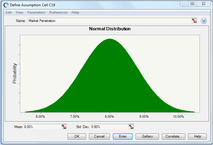
The marketing department estimates that Vision Research’s eventual share of the total market for the product will be normally distributed around a mean value of 8% with a standard deviation of 2%. “Normally distributed” means that Vision Research expects to see the familiar bell-shaped curve with about 68% of all possible values for market penetration falling between one standard deviation below the mean value and one standard deviation above the mean value, or between 6% and 10%.
In addition, the marketing department estimates a minimum market of 5%, given the interest shown in the product during preliminary testing.
Vision Research selects the normal distribution to describe the variable “market penetration.”
To define the assumption cell for market penetration:
In the Distribution Gallery, click the normal distribution.
(Scroll up to the top of the All category or click Basic to immediately display the normal distribution.)
The Normal Distribution dialog opens (Figure 120, Normal Distribution for Cell C19).
Specify the parameters for the normal distribution: the mean and the standard deviation.
The normal distribution scales to fit the chart area, so the shape of the distribution does not change. However, the scale of percentages on the chart axis does change.
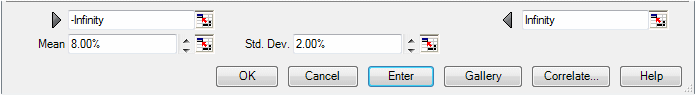
Click the More button,
 , to display additional text boxes (Figure 121, Assumption Truncation Text Boxes).
 These text boxes, marked by gray arrows, display the minimum and maximum values of the assumption range. If values are entered into them, they cut or truncate the range. These text boxes are then called the truncation minimum and maximum.
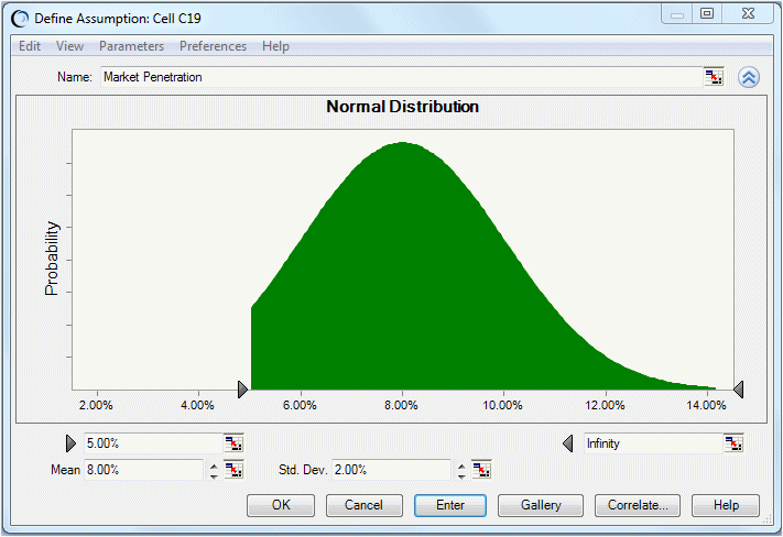
Type 5% in the minimum truncation text box (the first or left text box).
The distribution changes to reflect the values you entered (Figure 122, Changed Distribution for the Truncated Values).
When you run the simulation, Crystal Ball generates random values that follow a normal distribution around the mean value of 8%, and with no values generated below the 5% minimum limit.