4 Building Models in Oracle R Enterprise
Oracle R Enterprise provides functions for building regression models, neural network models, and models based on Oracle Data Mining algorithms.
This chapter has the following topics:
Building Oracle R Enterprise Models
The Oracle R Enterprise package OREmodels contains functions with which you can create advanced analytical data models using ore.frame objects, as described in the following topics:
About OREmodels Functions
The OREmodels package contains functions with which you can build advanced analytical data models using ore.frame objects. The OREmodels functions are the following:
Table 4-1 Functions in the OREmodels Package
| Function | Description |
|---|---|
|
|
Fits and uses a generalized linear model on data in an |
|
|
Fits a linear regression model on data in an |
|
|
Fits a neural network model on data in an |
|
|
Fits a stepwise linear regression model on data in an |
Note:
In R terminology, the phrase "fits a model" is often synonymous with "builds a model". In this document and in the online help for Oracle R Enterprise functions, the phrases are used interchangeably.The ore.glm, ore.lm, and ore.stepwise functions have the following advantages:
-
The algorithms provide accurate solutions using out-of-core QR factorization. QR factorization decomposes a matrix into an orthogonal matrix and a triangular matrix.
QR is an algorithm of choice for difficult rank-deficient models.
-
You can process data that does not fit into memory, that is, out-of-core data. QR factors a matrix into two matrices, one of which fits into memory while the other is stored on disk.
The
ore.glm,ore.lmandore.stepwisefunctions can solve data sets with more than one billion rows. -
The
ore.stepwisefunction allows fast implementations of forward, backward, and stepwise model selection techniques.
The ore.neural function has the following advantages:
-
It is a highly scalable implementation of neural networks, able to build a model on even billion row data sets in a matter of minutes. The
ore.neuralfunction can be run in two modes: in-memory for small to medium data sets and distributed (out-of-core) for large inputs. -
Users can specify the activation functions on neurons on a per-layer basis;
ore.neuralsupports many different activation functions. -
Users can specify a neural network topology consisting of any number of hidden layers, including none.
About the longley Data Set for Examples
Most of the linear regression and ore.neural examples use the longley data set, which is provided by R. It is a small macroeconomic data set that provides a well-known example for collinear regression and consists of seven economic variables observed yearly over 16 years.
Example 4-1 pushes the longley data set to a temporary database table that has the proxy ore.frame object longley_of displays the first six rows of longley_of.
Example 4-1 Displaying Values from the longley Data Set
longley_of <- ore.push(longley)
head(longley_of)
Listing for Example 4-1
R> longley_of <- ore.push(longley)
R> dim(longley_of)[1] 16  7
R> head(longley_of)
     GNP.deflator     GNP Unemployed Armed.Forces Population Year Employed
1947         83.0 234.289      235.6        159.0    107.608 1947   60.323
1948         88.5 259.426      232.5        145.6    108.632 1948   61.122
1949         88.2 258.054      368.2        161.6    109.773 1949   60.171
1950         89.5 284.599      335.1        165.0    110.929 1950   61.187
1951         96.2 328.975      209.9        309.9    112.075 1951   63.221
1952         98.1 346.999      193.2        359.4    113.270 1952   63.639
Building Linear Regression Models
The ore.lm and ore.stepwise functions perform least squares regression and stepwise least squares regression, respectively, on data represented in an ore.frame object. A model fit is generated using embedded R map/reduce operations where the map operation creates either QR decompositions or matrix cross-products depending on the number of coefficients being estimated. The underlying model matrices are created using either a model.matrix or sparse.model.matrix object depending on the sparsity of the model. Once the coefficients for the model have been estimated another pass of the data is made to estimate the model-level statistics.
When forward, backward, or stepwise selection is performed, the XtX and Xty matrices are subsetted to generate the F-test p-values based upon coefficient estimates that were generated using a Choleski decomposition of the XtX subset matrix.
If there are collinear terms in the model, functions ore.lm and ore.stepwise do not estimate the coefficient values for a collinear set of terms. For ore.stepwise, a collinear set of terms is excluded throughout the procedure.
For more information on ore.lm and ore.stepwise, invoke help(ore.lm).
Example 4-2 pushes the longley data set to a temporary database table that has the proxy ore.frame object longley_of. The example builds a linear regression model using ore.lm.
longley_of <- ore.push(longley)
# Fit full model
oreFit1 <- ore.lm(Employed ~ ., data = longley_of)
class(oreFit1)
summary(oreFit1)
Listing for Example 4-2
R> longley_of <- ore.push(longley)
R> # Fit full model
R>  oreFit1 <- ore.lm(Employed ~ ., data = longley_of)
R> class(oreFit1)
[1] "ore.lm"    "ore.model" "lm"
R> summary(oreFit1)

Call:
ore.lm(formula = Employed ~ ., data = longley_of)

Residuals:
     Min       1Q   Median       3Q      Max
-0.41011 -0.15767 -0.02816  0.10155  0.45539

Coefficients:
               Estimate Std. Error t value Pr(>|t|)
(Intercept)  -3.482e+03  8.904e+02  -3.911 0.003560 **
GNP.deflator  1.506e-02  8.492e-02   0.177 0.863141
GNP          -3.582e-02  3.349e-02  -1.070 0.312681
Unemployed   -2.020e-02  4.884e-03  -4.136 0.002535 **
Armed.Forces -1.033e-02  2.143e-03  -4.822 0.000944 ***
Population   -5.110e-02  2.261e-01  -0.226 0.826212
Year          1.829e+00  4.555e-01   4.016 0.003037 **
---
Signif. codes:  0 '***' 0.001 '**' 0.01 '*' 0.05 '.' 0.1 ' ' 1

Residual standard error: 0.3049 on 9 degrees of freedom
Multiple R-squared:  0.9955,    Adjusted R-squared:  0.9925
F-statistic: 330.3 on 6 and 9 DF,  p-value: 4.984e-10
Example 4-3 pushes the longley data set to a temporary database table that has the proxy ore.frame object longley_of. The example builds linear regression models using the ore.stepwise function.
Example 4-3 Using the ore.stepwise Function
longley_of <- ore.push(longley)
# Two stepwise alternatives
oreStep1 <-
  ore.stepwise(Employed ~ .^2, data = longley_of, add.p = 0.1, drop.p = 0.1)
oreStep2 <-
  step(ore.lm(Employed ~ 1, data = longley_of),
             scope = terms(Employed ~ .^2, data = longley_of))
Listing for Example 4-3
R> longley_of <- ore.push(longley)
R> # Two stepwise alternatives
R> oreStep1 <-
+   ore.stepwise(Employed ~ .^2, data = longley_of, add.p = 0.1, drop.p = 0.1)
R> oreStep2 <-
+   step(ore.lm(Employed ~ 1, data = longley_of),
+               scope = terms(Employed ~ .^2, data = longley_of))
Start:  AIC=41.17
Employed ~ 1

               Df Sum of Sq     RSS     AIC
+ GNP           1   178.973   6.036 -11.597
+ Year          1   174.552  10.457  -2.806
+ GNP.deflator  1   174.397  10.611  -2.571
+ Population    1   170.643  14.366   2.276
+ Unemployed    1    46.716 138.293  38.509
+ Armed.Forces  1    38.691 146.318  39.411
<none>                      185.009  41.165

Step:  AIC=-11.6
Employed ~ GNP

               Df Sum of Sq     RSS     AIC
+ Unemployed    1     2.457   3.579 -17.960
+ Population    1     2.162   3.874 -16.691
+ Year          1     1.125   4.911 -12.898
<none>                        6.036 -11.597
+ GNP.deflator  1     0.212   5.824 -10.169
+ Armed.Forces  1     0.077   5.959  -9.802
- GNP           1   178.973 185.009  41.165
... The rest of the output is not shown.
Building a Generalized Linear Model
The ore.glm functions fits generalized linear models on data in an ore.frame object. The function uses a Fisher scoring iteratively reweighted least squares (IRLS) algorithm.
Instead of the traditional step halving to prevent the selection of less optimal coefficient estimates, ore.glm uses a line search to select new coefficient estimates at each iteration, starting from the current coefficient estimates and moving through the Fisher scoring suggested estimates using the formula (1 - alpha) * old + alpha * suggested where alpha in [0, 2]. When the interp control argument is TRUE, the deviance is approximated by a cubic spline interpolation. When it is FALSE, the deviance is calculated using a follow-up data scan.
Each iteration consists of two or three embedded R execution map/reduce operations: an IRLS operation, an initial line search operation, and, if interp = FALSE, an optional follow-up line search operation. As with ore.lm, the IRLS map operation creates QR decompositions when update = "qr" or cross-products when update = "crossprod" of the model.matrix, or sparse.model.matrix if argument sparse = TRUE, and the IRLS reduce operation block updates those QR decompositions or cross-product matrices. After the algorithm has either converged or reached the maximum number of iterations, a final embedded R map/reduce operation is used to generate the complete set of model-level statistics.
The ore.glm function returns an ore.glm object.
For information on the ore.glm function arguments, invoke help(ore.glm).
Example 4-4 loads the rpart package and then pushes the kyphosis data set to a temporary database table that has the proxy ore.frame object KYPHOSIS. The example builds a generalized linear model using the ore.glm function and one using the glm function and invokes the summary function on the models.
Example 4-4 Using the ore.glm Function
# Load the rpart library to get the kyphosis and solder data sets.
library(rpart)
# Logistic regression
KYPHOSIS <- ore.push(kyphosis)
kyphFit1 <- ore.glm(Kyphosis ~ ., data = KYPHOSIS, family = binomial())
kyphFit2 <- glm(Kyphosis ~ ., data = kyphosis, family = binomial())
summary(kyphFit1)
summary(kyphFit2)
Listing for Example 4-4
R> # Load the rpart library to get the kyphosis and solder data sets.
R> library(rpart)

R> # Logistic regression
R> KYPHOSIS <- ore.push(kyphosis)
R> kyphFit1 <- ore.glm(Kyphosis ~ ., data = KYPHOSIS, family = binomial())
R> kyphFit2 <- glm(Kyphosis ~ ., data = kyphosis, family = binomial())
R> summary(kyphFit1)

Call:
ore.glm(formula = Kyphosis ~ ., data = KYPHOSIS, family = binomial())

Deviance Residuals:
    Min       1Q   Median       3Q      Max
-2.3124  -0.5484  -0.3632  -0.1659   2.1613

Coefficients:
             Estimate Std. Error z value Pr(>|z|)
(Intercept) -2.036934   1.449622  -1.405  0.15998
Age          0.010930   0.006447   1.696  0.08997 .
Number       0.410601   0.224870   1.826  0.06786 .
Start       -0.206510   0.067700  -3.050  0.00229 **
---
Signif. codes:  0 '***' 0.001 '**' 0.01 '*' 0.05 '.' 0.1 ' ' 1

(Dispersion parameter for binomial family taken to be 1)

    Null deviance: 83.234  on 80  degrees of freedom
Residual deviance: 61.380  on 77  degrees of freedom
AIC: 69.38

Number of Fisher Scoring iterations: 4

R> summary(kyphFit2)

Call:
glm(formula = Kyphosis ~ ., family = binomial(), data = kyphosis)

Deviance Residuals:
    Min       1Q   Median       3Q      Max
-2.3124  -0.5484  -0.3632  -0.1659   2.1613

Coefficients:
             Estimate Std. Error z value Pr(>|z|)
(Intercept) -2.036934   1.449575  -1.405  0.15996
Age          0.010930   0.006446   1.696  0.08996 .
Number       0.410601   0.224861   1.826  0.06785 .
Start       -0.206510   0.067699  -3.050  0.00229 **
---
Signif. codes:  0 '***' 0.001 '**' 0.01 '*' 0.05 '.' 0.1 ' ' 1

(Dispersion parameter for binomial family taken to be 1)

    Null deviance: 83.234  on 80  degrees of freedom
Residual deviance: 61.380  on 77  degrees of freedom
AIC: 69.38

Number of Fisher Scoring iterations: 5

# Poisson regression
R> SOLDER <- ore.push(solder)
R> solFit1 <- ore.glm(skips ~ ., data = SOLDER, family = poisson())
R> solFit2 <- glm(skips ~ ., data = solder, family = poisson())
R> summary(solFit1)

Call:
ore.glm(formula = skips ~ ., data = SOLDER, family = poisson())

Deviance Residuals:
    Min       1Q   Median       3Q      Max
-3.4105  -1.0897  -0.4408   0.6406   3.7927

Coefficients:
            Estimate Std. Error z value Pr(>|z|)
(Intercept) -1.25506    0.10069 -12.465  < 2e-16 ***
OpeningM     0.25851    0.06656   3.884 0.000103 ***
OpeningS     1.89349    0.05363  35.305  < 2e-16 ***
SolderThin   1.09973    0.03864  28.465  < 2e-16 ***
MaskA3       0.42819    0.07547   5.674 1.40e-08 ***
MaskB3       1.20225    0.06697  17.953  < 2e-16 ***
MaskB6       1.86648    0.06310  29.580  < 2e-16 ***
PadTypeD6   -0.36865    0.07138  -5.164 2.41e-07 ***
PadTypeD7   -0.09844    0.06620  -1.487 0.137001
PadTypeL4    0.26236    0.06071   4.321 1.55e-05 ***
PadTypeL6   -0.66845    0.07841  -8.525  < 2e-16 ***
PadTypeL7   -0.49021    0.07406  -6.619 3.61e-11 ***
PadTypeL8   -0.27115    0.06939  -3.907 9.33e-05 ***
PadTypeL9   -0.63645    0.07759  -8.203 2.35e-16 ***
PadTypeW4   -0.11000    0.06640  -1.657 0.097591 .
PadTypeW9   -1.43759    0.10419 -13.798  < 2e-16 ***
Panel        0.11818    0.02056   5.749 8.97e-09 ***
---
Signif. codes:  0 '***' 0.001 '**' 0.01 '*' 0.05 '.' 0.1 ' ' 1

(Dispersion parameter for poisson family taken to be 1)

    Null deviance: 6855.7  on 719  degrees of freedom
Residual deviance: 1165.4  on 703  degrees of freedom
AIC: 2781.6

Number of Fisher Scoring iterations: 4
Building a Neural Network Model
Neural network models can be used to capture intricate nonlinear relationships between inputs and outputs or to find patterns in data. The ore.neural function builds a feed-forward neural network for regression on ore.frame data. It supports multiple hidden layers with a specifiable number of nodes. Each layer can have one of several activation functions.
The output layer is a single numeric or binary categorical target. The output layer can have any of the activation functions. It has the linear activation function by default.
The output of ore.neural is an object of type ore.neural.
Modeling with the ore.neural function is well-suited for noisy and complex data such as sensor data. Problems that such data might have are the following:
-
Potentially many (numeric) predictors, for example, pixel values
-
The target may be discrete-valued, real-valued, or a vector of such values
-
Training data may contain errors – robust to noise
-
Fast scoring
-
Model transparency is not required; models difficult to interpret
Typical steps in neural network modeling are the following:
-
Specifying the architecture
-
Preparing the data
-
Building the model
-
Specifying the stopping criteria: iterations, error on a validation set within tolerance
-
Viewing statistical results from model
-
Improving the model
For information about the arguments to the ore.neural function, invoke help(ore.neural).
Example 4-5 builds a neural network with default values, including a hidden size of 1. The example pushes a subset of the longley data set to an ore.frame object in database memory as the object trainData. The example then pushes a different subset of longley to the database as the object testData. The example builds a neural network model with trainData and then predicts results using testData.
Example 4-5 Building a Neural Network Model
trainData <- ore.push(longley[1:11, ])
testData <- ore.push(longley[12:16, ])
fit <- ore.neural('Employed ~ GNP + Population + Year', data = trainData)
ans <- predict(fit, newdata = testData)
ans
Listing for Example 4-5
R> trainData <- ore.push(longley[1:11, ])
R> testData <- ore.push(longley[12:16, ])
R> fit <- ore.neural('Employed ~ GNP + Population + Year', data = trainData)
R> ans <- predict(fit, newdata = testData)
R> ans
  pred_Employed
1      67.97452
2      69.50893
3      70.28098
4      70.86127
5      72.31066
Warning message:
ORE object has no unique key - using random order
Example 4-6 pushes the iris data set to a temporary database table that has the proxy ore.frame object IRIS. The example builds a neural network model using the ore.neural function and specifies a different activation function for each layer.
Example 4-6 Using ore.neural and Specifying Activations
IRIS <- ore.push(iris)
fit <- ore.neural(Petal.Length ~ Petal.Width + Sepal.Length,
                  data = IRIS,
                  sparse = FALSE,
                  hiddenSizes = c(20, 5),
                  activations = c("bSigmoid", "tanh", "linear"))
ans <- predict(fit, newdata = IRIS,
               supplemental.cols = c("Petal.Length"))
options(ore.warn.order = FALSE)
head(ans, 3)
summary(ans)
Listing for Example 4-6
R> IRIS <- ore.push(iris)
R> fit <- ore.neural(Petal.Length ~ Petal.Width + Sepal.Length,
+                   data = IRIS,
+                   sparse = FALSE,
+                   hiddenSizes = c(20, 5),
+                   activations = c("bSigmoid", "tanh", "linear"))
R>
R> ans <- predict(fit, newdata = IRIS,
+                supplemental.cols = c("Petal.Length"))
R> options(ore.warn.order = FALSE)
R> head(ans, 3)
  Petal.Length pred_Petal.Length
1          1.4          1.416466
2          1.4          1.363385
3          1.3          1.310709
R> summary(ans)
  Petal.Length   pred_Petal.Length
 Min.   :1.000   Min.   :1.080
 1st Qu.:1.600   1st Qu.:1.568
 Median :4.350   Median :4.346
 Mean   :3.758   Mean   :3.742
 3rd Qu.:5.100   3rd Qu.:5.224
 Max.   :6.900   Max.   :6.300
Building Oracle Data Mining Models
This section describes using the functions in the OREdm package of Oracle R Enterprise to build Oracle Data Mining models in R. The section has the following topics:
See Also:
Oracle Data Mining ConceptsAbout Building Oracle Data Mining Models using Oracle R Enterprise
Oracle Data Mining can mine tables, views, star schemas, transactional data, and unstructured data. The OREdm functions provide R interfaces that use arguments that conform to typical R usage for corresponding predictive analytics and data mining functions.
This section has the following topics:
Oracle Data Mining Models Supported by Oracle R Enterprise
The functions in the OREdm package provide access to the in-database data mining functionality of Oracle Database. You use these functions to build data mining models in the database.
Table 4-2 lists the Oracle R Enterprise functions that build Oracle Data Mining models and the corresponding Oracle Data Mining algorithms and functions.
Table 4-2 Oracle R Enterprise Data Mining Model Functions
| Oracle R Enterprise Function | Oracle Data Mining Algorithm | Oracle Data Mining Function |
|---|---|---|
|
|
Minimum Description Length |
Attribute Importance for Classification or Regression |
|
|
Apriori |
Association Rules |
|
|
Decision Tree |
Classification |
|
|
Generalized Linear Models |
Classification and Regression |
|
|
k-Means |
Clustering |
|
|
Naive Bayes |
Classification |
|
|
Non-Negative Matrix Factorization |
Feature Extraction |
|
|
Orthogonal Partitioning Cluster (O-Cluster) |
Clustering |
|
|
Support Vector Machines |
Classification and Regression |
About Oracle Data Mining Models Built by Oracle R Enterprise Functions
In each OREdm R model object, the slot name (or fit.name) is the name of the underlying Oracle Data Mining model generated by the OREdm function. While the R model exists, the Oracle Data Mining model name can be used to access the Oracle Data Mining model through other interfaces, including:
-
Oracle Data Miner
-
Any SQL interface, such as SQL*Plus or SQL Developer
In particular, the models can be used with the Oracle Data Mining SQL prediction functions.
With Oracle Data Miner you can do the following:
-
Get a list of available models
-
Use model viewers to inspect model details
-
Score appropriately transformed data
Note:
Any transformations performed in the R space are not carried over into Oracle Data Miner or SQL scoring.Users can also get a list of models using SQL for inspecting model details or for scoring appropriately transformed data.
Models built using OREdm functions are transient objects; they do not persist past the R session in which they were built unless they are explicitly saved in an Oracle R Enterprise datastore. Oracle Data Mining models built using Data Miner or SQL, on the other hand, exist until they are explicitly dropped.
Model objects can be saved or persisted, as described in "Saving and Managing R Objects in the Database". Saving a model object generated by an OREdm function allows it to exist across R sessions and keeps the corresponding Oracle Data Mining object in place. While the OREdm model exists, you can export and import it; then you can use it apart from the Oracle R Enterprise R object existence.
Building an Association Rules Model
The ore.odmAssocRules function implements the apriori algorithm to find frequent itemsets and generate an association model. It finds the co-occurrence of items in large volumes of transactional data such as in the case of market basket analysis. An association rule identifies a pattern in the data in which the appearance of a set of items in a transactional record implies another set of items. The groups of items used to form rules must pass a minimum threshold according to how frequently they occur (the support of the rule) and how often the consequent follows the antecedent (the confidence of the rule). Association models generate all rules that have support and confidence greater than user-specified thresholds. The apriori algorithm is efficient, and scales well with respect to the number of transactions, number of items, and number of itemsets and rules produced.
The formula specification has the form ~ terms, where terms is a series of column names to include in the analysis. Multiple column names are specified using + between column names. Use ~ . if all columns in data should be used for model building. To exclude columns, use - before each column name to exclude. Functions can be applied to the items in terms to realize transformations.
The ore.odmAssocRules function accepts data in the following forms:
-
Transactional data
-
Multi-record case data using item id and item value
-
Relational data
For examples of specifying the forms of data and for information on the arguments of the function, invoke help(ore.odmAssocRules).
The function rules returns an object of class ore.rules, which specifies a set of association rules. You can pull an ore.rules object into memory in a local R session by using ore.pull. The local in-memory object is of class rules defined in the arules package. See help(ore.rules).
The function itemsets returns an object of class ore.itemsets, which specifies a set of itemsets. You can pull an ore.itemsets object into memory in a local R session by using ore.pull. The local in-memory object is of class itemsets defined in the arules package. See help(ore.itemsets).
Example 4-7 builds an association model on a transactional data set. The packages arules and arulesViz are required to pull the resulting rules and itemsets into the client R session memory and be visualized. The graph of the rules appears in Figure 4-1.
Example 4-7 Using the ore.odmAssocRules Function
# Load the arules and arulesViz packages.
library(arules)
library(arulesViz)
# Create some transactional data.
id <- c(1, 1, 1, 2, 2, 2, 2, 3, 3, 3, 3)
item <- c("b", "d", "e", "a", "b", "c", "e", "b", "c", "d", "e")
# Push the data to the database as an ore.frame object.
transdata_of <- ore.push(data.frame(ID = id, ITEM = item))
# Build a model with specifications.
ar.mod1 <- ore.odmAssocRules(~., transdata_of, case.id.column = "ID",
             item.id.column = "ITEM", min.support = 0.6, min.confidence = 0.6,
             max.rule.length = 3)
# Generate itemsets and rules of the model.
itemsets <- itemsets(ar.mod1)
rules <- rules(ar.mod1)
# Convert the rules to the rules object in arules package.
rules.arules <- ore.pull(rules)
inspect(rules.arules)
# Convert itemsets to the itemsets object in arules package.
itemsets.arules <- ore.pull(itemsets)
inspect(itemsets.arules)
# Plot the rules graph.
plot(rules.arules, method = "graph", interactive = TRUE)
Listing for Example 4-7
R> # Load the arules and arulesViz packages.
R> library(arules)
R> library(arulesViz)
R> # Create some transactional data.
R> id <- c(1, 1, 1, 2, 2, 2, 2, 3, 3, 3, 3)
R> item <- c("b", "d", "e", "a", "b", "c", "e", "b", "c", "d", "e")
R> # Push the data to the database as an ore.frame object.
R> transdata_of <- ore.push(data.frame(ID = id, ITEM = item))
R> # Build a model with specifications.
R> ar.mod1 <- ore.odmAssocRules(~., transdata_of, case.id.column = "ID",
+             item.id.column = "ITEM", min.support = 0.6, min.confidence = 0.6,
+             max.rule.length = 3)
R> # Generate itemsets and rules of the model.
R> itemsets <- itemsets(ar.mod1)
R> rules <- rules(ar.mod1)
R> # Convert the rules to the rules object in arules package.
R> rules.arules <- ore.pull(rules)
R> inspect(rules.arules)
   lhs    rhs   support confidence lift
1  {b} => {e} 1.0000000  1.0000000    1
2  {e} => {b} 1.0000000  1.0000000    1
3  {c} => {e} 0.6666667  1.0000000    1
4  {d,
    e} => {b} 0.6666667  1.0000000    1
5  {c,
    e} => {b} 0.6666667  1.0000000    1
6  {b,
    d} => {e} 0.6666667  1.0000000    1
7  {b,
    c} => {e} 0.6666667  1.0000000    1
8  {d} => {b} 0.6666667  1.0000000    1
9  {d} => {e} 0.6666667  1.0000000    1
10 {c} => {b} 0.6666667  1.0000000    1
11 {b} => {d} 0.6666667  0.6666667    1
12 {b} => {c} 0.6666667  0.6666667    1
13 {e} => {d} 0.6666667  0.6666667    1
14 {e} => {c} 0.6666667  0.6666667    1
15 {b,
    e} => {d} 0.6666667  0.6666667    1
16 {b,
    e} => {c} 0.6666667  0.6666667    1
R> # Convert itemsets to the itemsets object in arules package.
R> itemsets.arules <- ore.pull(itemsets)
R> inspect(itemsets.arules)
   items   support
1  {b}   1.0000000
2  {e}   1.0000000
3  {b,
    e}   1.0000000
4  {c}   0.6666667
5  {d}   0.6666667
6  {b,
    c}   0.6666667
7  {b,
    d}   0.6666667
8  {c,
    e}   0.6666667
9  {d,
    e}   0.6666667
10 {b,
    c,
    e}   0.6666667
11 {b,
    d,
    e}   0.6666667

R> # Plot the rules graph.
R> plot(rules.arules, method = "graph", interactive = TRUE)
Figure 4-1 A Visual Demonstration of the Association Rules
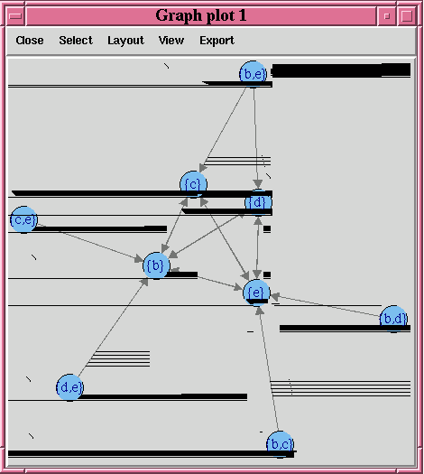
Description of "Figure 4-1 A Visual Demonstration of the Association Rules"
Building an Attribute Importance Model
The ore.odmAI function uses the Oracle Data Mining Minimum Description Length algorithm to calculate attribute importance. Attribute importance ranks attributes according to their significance in predicting a target.
Minimum Description Length (MDL) is an information theoretic model selection principle. It is an important concept in information theory (the study of the quantification of information) and in learning theory (the study of the capacity for generalization based on empirical data).
MDL assumes that the simplest, most compact representation of the data is the best and most probable explanation of the data. The MDL principle is used to build Oracle Data Mining attribute importance models.
Attribute Importance models built using Oracle Data Mining cannot be applied to new data.
The ore.odmAI function produces a ranking of attributes and their importance values.
Note:
OREdm AI models differ from Oracle Data Mining AI models in these ways: a model object is not retained, and an R model object is not returned. Only the importance ranking created by the model is returned.For information on the ore.odmAI function arguments, invoke help(ore.odmAI).
Example 4-8 pushes the data.frame iris to the database as the ore.frame iris_of. The example then builds an attribute importance model.
Listing for Example 4-8
R> iris_of <- ore.push(iris)
R> ore.odmAI(Species ~ ., iris_of)

Call:
ore.odmAI(formula = Species ~ ., data = iris_of)

Importance:
             importance rank
Petal.Width   1.1701851    1
Petal.Length  1.1494402    2
Sepal.Length  0.5248815    3
Sepal.Width   0.2504077    4
Building a Decision Tree Model
The ore.odmDT function uses the Oracle Data Mining Decision Tree algorithm, which is based on conditional probabilities. Decision trees generate rules. A rule is a conditional statement that can easily be understood by humans and be used within a database to identify a set of records.
Decision Tree models are classification models.
A decision tree predicts a target value by asking a sequence of questions. At a given stage in the sequence, the question that is asked depends upon the answers to the previous questions. The goal is to ask questions that, taken together, uniquely identify specific target values. Graphically, this process forms a tree structure.
During the training process, the Decision Tree algorithm must repeatedly find the most efficient way to split a set of cases (records) into two child nodes. The ore.odmDT function offers two homogeneity metrics, gini and entropy, for calculating the splits. The default metric is gini.
For information on the ore.odmDT function arguments, invoke help(ore.odmDT).
Example 4-9 creates an input ore.frame, builds a model, makes predictions, and generates a confusion matrix.
Example 4-9 Using the ore.odmDT Function
m <- mtcars
m$gear <- as.factor(m$gear)
m$cyl  <- as.factor(m$cyl)
m$vs   <- as.factor(m$vs)
m$ID   <- 1:nrow(m)
mtcars_of <- ore.push(m)
row.names(mtcars_of) <- mtcars_of
# Build the model.
dt.mod  <- ore.odmDT(gear ~ ., mtcars_of)
summary(dt.mod)
# Make predictions and generate a confusion matrix.
dt.res  <- predict (dt.mod, mtcars_of, "gear")
with(dt.res, table(gear, PREDICTION))
Listing for Example 4-9
R> m <- mtcars
R> m$gear <- as.factor(m$gear)
R> m$cyl  <- as.factor(m$cyl)
R> m$vs   <- as.factor(m$vs)
R> m$ID   <- 1:nrow(m)
R> mtcars_of <- ore.push(m)
R> row.names(mtcars_of) <- mtcars_of
R> # Build the model.
R> dt.mod  <- ore.odmDT(gear ~ ., mtcars_of)
R> summary(dt.mod)

Call:
ore.odmDT(formula = gear ~ ., data = mtcars_of)

  n =  32

Nodes:
  parent node.id row.count prediction                         split
1     NA       0        32          3                          <NA>
2      0       1        16          4 (disp <= 196.299999999999995)
3      0       2        16          3  (disp > 196.299999999999995)
            surrogate                   full.splits
1                <NA>                          <NA>
2 (cyl in ("4" "6" )) (disp <= 196.299999999999995)
3     (cyl in ("8" ))  (disp > 196.299999999999995)

Settings:
                          value
prep.auto                    on
impurity.metric   impurity.gini
term.max.depth                7
term.minpct.node           0.05
term.minpct.split           0.1
term.minrec.node             10
term.minrec.split            20
R> # Make predictions and generate a confusion matrix.
R> dt.res  <- predict (dt.mod, mtcars_of, "gear")
R> with(dt.res, table(gear, PREDICTION))
    PREDICTION
gear  3  4
   3 14  1
   4  0 12
   5  2  3
Building General Linearized Models
The ore.odmGLM function builds Generalized Linear Models (GLM), which include and extend the class of linear models (linear regression). Generalized linear models relax the restrictions on linear models, which are often violated in practice. For example, binary (yes/no or 0/1) responses do not have same variance across classes.
The Oracle Data Mining GLM is a parametric modeling technique. Parametric models make assumptions about the distribution of the data. When the assumptions are met, parametric models can be more efficient than non-parametric models.
The challenge in developing models of this type involves assessing the extent to which the assumptions are met. For this reason, quality diagnostics are key to developing quality parametric models.
In addition to the classical weighted least squares estimation for linear regression and iteratively re-weighted least squares estimation for logistic regression, both solved through Cholesky decomposition and matrix inversion, Oracle Data Mining GLM provides a conjugate gradient-based optimization algorithm that does not require matrix inversion and is very well suited to high-dimensional data. The choice of algorithm is handled internally and is transparent to the user.
GLM can be used to build classification or regression models as follows:
-
Classification: Binary logistic regression is the GLM classification algorithm. The algorithm uses the logit link function and the binomial variance function.
-
Regression: Linear regression is the GLM regression algorithm. The algorithm assumes no target transformation and constant variance over the range of target values.
The ore.odmGLM function allows you to build two different types of models. Some arguments apply to classification models only and some to regression models only.
For information on the ore.odmGLM function arguments, invoke help(ore.odmGLM).
The following examples build several models using GLM. The input ore.frame objects are R data sets pushed to the database.
Example 4-10 builds a linear regression model using the longley data set.
Example 4-10 Building a Linear Regression Model
longley_of <- ore.push(longley)
longfit1 <- ore.odmGLM(Employed ~ ., data = longley_of)
summary(longfit1)
Listing for Example 4-10
R> longley_of <- ore.push(longley)
R> longfit1 <- ore.odmGLM(Employed ~ ., data = longley_of)
R> summary(longfit1)

Call:
ore.odmGLM(formula = Employed ~ ., data = longely_of)

Residuals:
     Min       1Q   Median       3Q      Max
-0.41011 -0.15767 -0.02816  0.10155  0.45539

Coefficients:
               Estimate Std. Error t value Pr(>|t|)
(Intercept)  -3.482e+03  8.904e+02  -3.911 0.003560 **
GNP.deflator  1.506e-02  8.492e-02   0.177 0.863141
GNP          -3.582e-02  3.349e-02  -1.070 0.312681
Unemployed   -2.020e-02  4.884e-03  -4.136 0.002535 **
Armed.Forces -1.033e-02  2.143e-03  -4.822 0.000944 ***
Population   -5.110e-02  2.261e-01  -0.226 0.826212
Year          1.829e+00  4.555e-01   4.016 0.003037 **
---
Signif. codes:  0 '***' 0.001 '**' 0.01 '*' 0.05 '.' 0.1 ' ' 1

Residual standard error: 0.3049 on 9 degrees of freedom
Multiple R-squared:  0.9955,    Adjusted R-squared:  0.9925
F-statistic: 330.3 on 6 and 9 DF,  p-value: 4.984e-10
Example 4-11 uses the longley_of ore.frame from Example 4-10. Example 4-11 invokes the ore.odmGLM function and specifies using ridge estimation for the coefficients.
Example 4-11 Using Ridge Estimation for the Coefficients of the ore.odmGLM Model
longfit2 <- ore.odmGLM(Employed ~ ., data = longley_of, ridge = TRUE,
                       ridge.vif = TRUE)
summary(longfit2)
Listing for Example 4-11
R> longfit2 <- ore.odmGLM(Employed ~ ., data = longley_of, ridge = TRUE,
+                         ridge.vif = TRUE)
R> summary(longfit2)

Call:
ore.odmGLM(formula = Employed ~ ., data = longley_of, ridge = TRUE,
    ridge.vif = TRUE)

Residuals:
    Min      1Q  Median      3Q     Max
-0.4100 -0.1579 -0.0271  0.1017  0.4575

Coefficients:
               Estimate   VIF
(Intercept)  -3.466e+03 0.000
GNP.deflator  1.479e-02 0.077
GNP          -3.535e-02 0.012
Unemployed   -2.013e-02 0.000
Armed.Forces -1.031e-02 0.000
Population   -5.262e-02 0.548
Year          1.821e+00 2.212

Residual standard error: 0.3049 on 9 degrees of freedom
Multiple R-squared:  0.9955,    Adjusted R-squared:  0.9925
F-statistic: 330.2 on 6 and 9 DF,  p-value: 4.986e-10
Example 4-12 builds a logistic regression (classification) model. It uses the infert data set. The example invokes the ore.odmGLM function and specifies logistic as the type argument, which builds a binomial GLM.
Example 4-12 Building a Logistic Regression GLM
infert_of <- ore.push(infert)
infit1 <- ore.odmGLM(case ~ age+parity+education+spontaneous+induced,
                     data = infert_of, type = "logistic")
infit1
Listing for Example 4-12
R> infert_of <- ore.push(infert)
R> infit1 <- ore.odmGLM(case ~ age+parity+education+spontaneous+induced,
+                       data = infert_of, type = "logistic")
R> infit1

Response:
case == "1"

Call:  ore.odmGLM(formula = case ~ age + parity + education + spontaneous +
    induced, data = infert_of, type = "logistic")

Coefficients:
     (Intercept)               age            parity   education0-5yrs  education12+ yrs       spontaneous           induced
        -2.19348           0.03958          -0.82828           1.04424          -0.35896           2.04590           1.28876

Degrees of Freedom: 247 Total (i.e. Null);  241 Residual
Null Deviance:      316.2
Residual Deviance: 257.8        AIC: 271.8
Example 4-13 builds a logistic regression (classification) model and specifies a reference value. The example uses the infert_of ore.frame from Example 4-12.
Example 4-13 Specifying a Reference Value in Building a Logistic Regression GLM
infit2 <- ore.odmGLM(case ~ age+parity+education+spontaneous+induced,
                     data = infert_of, type = "logistic", reference = 1)
infit2
Listing for Example 4-13
infit2 <- ore.odmGLM(case ~ age+parity+education+spontaneous+induced,
                     data = infert_of, type = "logistic", reference = 1)
infit2

Response:
case == "0"

Call:  ore.odmGLM(formula = case ~ age + parity + education + spontaneous +
    induced, data = infert_of, type = "logistic", reference = 1)

Coefficients:
     (Intercept)               age            parity   education0-5yrs  education12+ yrs       spontaneous           induced
         2.19348          -0.03958           0.82828          -1.04424           0.35896          -2.04590          -1.28876

Degrees of Freedom: 247 Total (i.e. Null);  241 Residual
Null Deviance:      316.2
Residual Deviance: 257.8        AIC: 271.8
Building a k-Means Model
The ore.odmKM function uses the Oracle Data Mining k-Means (KM) algorithm, a distance-based clustering algorithm that partitions data into a specified number of clusters. The algorithm has the following features:
-
Several distance functions: Euclidean, Cosine, and Fast Cosine distance functions. The default is Euclidean.
-
For each cluster, the algorithm returns the centroid, a histogram for each attribute, and a rule describing the hyperbox that encloses the majority of the data assigned to the cluster. The centroid reports the mode for categorical attributes and the mean and variance for numeric attributes.
For information on the ore.odmKM function arguments, invoke help(ore.odmKM).
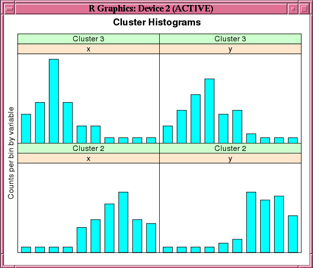
Example 4-14 demonstrates the use of the ore.odmKMeans function. The example creates two matrices that have 100 rows and two columns. The values in the rows are random variates. It binds the matrices into the matrix x. The example coerces x to a data.frame and pushes it to the database as x_of, an ore.frame object. The example invokes the ore.odmKMeans function to build the KM model, km.mod1. The example then invokes the summary and histogram functions on the model. Figure 4-2 shows the graphic displayed by the histogram function.
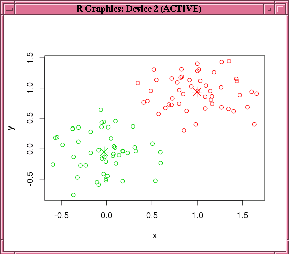
The example then makes a prediction using the model and pulls the result to local memory. It plots the results. Figure 4-3 shows the graphic displayed by the points function in the example.
Example 4-14 Using the ore.odmKM Function
x <- rbind(matrix(rnorm(100, sd = 0.3), ncol = 2),
           matrix(rnorm(100, mean = 1, sd = 0.3), ncol = 2))
colnames(x) <- c("x", "y")
x_of <- ore.push (data.frame(x))
km.mod1 <- NULL
km.mod1 <- ore.odmKMeans(~., x_of, num.centers=2)
summary(km.mod1)
histogram(km.mod1) # See Figure 4-2.
# Make a prediction.
km.res1 <- predict(km.mod1, x_of, type="class", supplemental.cols=c("x","y"))
head(km.res1, 3)
# Pull the results to the local memory and plot them.
km.res1.local <- ore.pull(km.res1)
plot(data.frame(x=km.res1.local$x, y=km.res1.local$y),
                col=km.res1.local$CLUSTER_ID)
points(km.mod1$centers2, col = rownames(km.mod1$centers2), pch = 8, cex=2)
head(predict(km.mod1, x_of, type=c("class","raw"),
             supplemental.cols=c("x","y")), 3)
Listing for Example 4-14
R> x <- rbind(matrix(rnorm(100, sd = 0.3), ncol = 2),
+             matrix(rnorm(100, mean = 1, sd = 0.3), ncol = 2))
R> colnames(x) <- c("x", "y")
R> x_of <- ore.push (data.frame(x))
R> km.mod1 <- NULL
R> km.mod1 <- ore.odmKMeans(~., x_of, num.centers=2)
R> summary(km.mod1)

Call:
ore.odmKMeans(formula = ~., data = x_of, num.centers = 2)

Settings:
                         value
clus.num.clusters            2
block.growth                 2
conv.tolerance            0.01
distance             euclidean
iterations                   3
min.pct.attr.support       0.1
num.bins                    10
split.criterion       variance
prep.auto                   on

Centers:
            x           y
2  0.99772307  0.93368684
3 -0.02721078 -0.05099784
R> histogram(km.mod1) # See Figure 4-2.
R> # Make a prediction.
R> km.res1 <- predict(km.mod1, x_of, type="class", supplemental.cols=c("x","y"))
R> head(km.res1, 3)
            x          y CLUSTER_ID
1 -0.03038444  0.4395409          3
2  0.17724606 -0.5342975          3
3 -0.17565761  0.2832132          3
# Pull the results to the local memory and plot them.
R> km.res1.local <- ore.pull(km.res1)
R> plot(data.frame(x=km.res1.local$x, y=km.res1.local$y),
+                  col=km.res1.local$CLUSTER_ID)
R> points(km.mod1$centers2, col = rownames(km.mod1$centers2), pch = 8, cex=2)
R> # See Figure 4-3.
R> head(predict(km.mod1, x_of, type=c("class","raw"),
                supplemental.cols=c("x","y")), 3)
           '2'       '3'           x          y CLUSTER_ID
1 8.610341e-03 0.9913897 -0.03038444  0.4395409          3
2 8.017890e-06 0.9999920  0.17724606 -0.5342975          3
3 5.494263e-04 0.9994506 -0.17565761  0.2832132          3
Figure 4-2 shows the graphic displayed by the invocation of the histogram function in Example 4-14.
Figure 4-2 Cluster Histograms for the km.mod1 Model
Description of "Figure 4-2 Cluster Histograms for the km.mod1 Model"
Figure 4-3 shows the graphic displayed by the invocation of the points function in Example 4-14.
Figure 4-3 Results of the points Function for the km.mod1 Model
Description of "Figure 4-3 Results of the points Function for the km.mod1 Model"
Building a Naive Bayes Model
The ore.odmNB function builds an Oracle Data Mining Naive Bayes model. The Naive Bayes algorithm is based on conditional probabilities. Naive Bayes looks at the historical data and calculates conditional probabilities for the target values by observing the frequency of attribute values and of combinations of attribute values.
Naive Bayes assumes that each predictor is conditionally independent of the others. (Bayes' Theorem requires that the predictors be independent.)
For information on the ore.odmNB function arguments, invoke help(ore.odmNB).
Example 4-15 creates an input ore.frame, builds a Naive Bayes model, makes predictions, and generates a confusion matrix.
Example 4-15 Using the ore.odmNB Function
m <- mtcars
m$gear <- as.factor(m$gear)
m$cyl  <- as.factor(m$cyl)
m$vs   <- as.factor(m$vs)
m$ID   <- 1:nrow(m)
mtcars_of <- ore.push(m)
row.names(mtcars_of) <- mtcars_of
# Build the model.
nb.mod  <- ore.odmNB(gear ~ ., mtcars_of)
summary(nb.mod)
# Make predictions and generate a confusion matrix.
nb.res  <- predict (nb.mod, mtcars_of, "gear")
with(nb.res, table(gear, PREDICTION))
Listing for Example 4-15
R> m <- mtcars
R> m$gear <- as.factor(m$gear)
R> m$cyl  <- as.factor(m$cyl)
R> m$vs   <- as.factor(m$vs)
R> m$ID   <- 1:nrow(m)
R> mtcars_of <- ore.push(m)
R> row.names(mtcars_of) <- mtcars_of
R> # Build the model.
R> nb.mod  <- ore.odmNB(gear ~ ., mtcars_of)
R> summary(nb.mod)

Call:
ore.odmNB(formula = gear ~ ., data = mtcars_of)

Settings:
          value
prep.auto    on

Apriori:
      3       4       5
0.46875 0.37500 0.15625
Tables:
$ID
  ( ; 26.5), [26.5; 26.5]  (26.5;  )
3              1.00000000
4              0.91666667 0.08333333
5                         1.00000000

$am
          0         1
3 1.0000000
4 0.3333333 0.6666667
5           1.0000000

$cyl
  '4', '6' '8'
3      0.2 0.8
4      1.0
5      0.6 0.4

$disp
  ( ; 196.299999999999995), [196.299999999999995; 196.299999999999995]
3                                                           0.06666667
4                                                           1.00000000
5                                                           0.60000000
  (196.299999999999995;  )
3               0.93333333
4
5               0.40000000

$drat
  ( ; 3.385), [3.385; 3.385] (3.385;  )
3                  0.8666667  0.1333333
4                             1.0000000
5                             1.0000000
$hp
  ( ; 136.5), [136.5; 136.5] (136.5;  )
3                        0.2        0.8
4                        1.0
5                        0.4        0.6

$vs
          0         1
3 0.8000000 0.2000000
4 0.1666667 0.8333333
5 0.8000000 0.2000000

$wt
  ( ; 3.2024999999999999), [3.2024999999999999; 3.2024999999999999]
3                                                        0.06666667
4                                                        0.83333333
5                                                        0.80000000
  (3.2024999999999999;  )
3              0.93333333
4              0.16666667
5              0.20000000


Levels:
[1] "3" "4" "5"

R> # Make predictions and generate a confusion matrix.
R> nb.res  <- predict (nb.mod, mtcars_of, "gear")
R> with(nb.res, table(gear, PREDICTION))
    PREDICTION
gear  3  4  5
   3 14  1  0
   4  0 12  0
   5  0  1  4
Building a Non-Negative Matrix Factorization Model
The ore.odmNMF function builds an Oracle Data Mining Non-Negative Matrix Factorization (NMF) model for feature extraction. Each feature extracted by NMF is a linear combination of the original attribution set. Each feature has a set of non-negative coefficients, which are a measure of the weight of each attribute on the feature. If the argument allow.negative.scores is TRUE, then negative coefficients are allowed.
For information on the ore.odmNMF function arguments, invoke help(ore.odmNMF).
Example 4-16 creates an NMF model on a training data set and scores on a test data set.
Example 4-16 Using the ore.odmNMF Function
training.set <- ore.push(npk[1:18, c("N","P","K")])
scoring.set <- ore.push(npk[19:24, c("N","P","K")])
nmf.mod <- ore.odmNMF(~., training.set, num.features = 3)
features(nmf.mod)
summary(nmf.mod)
predict(nmf.mod, scoring.set)
Listing for Example 4-16
R> training.set <- ore.push(npk[1:18, c("N","P","K")])
R> scoring.set <- ore.push(npk[19:24, c("N","P","K")])
R> nmf.mod <- ore.odmNMF(~., training.set, num.features = 3)
R> features(nmf.mod)
   FEATURE_ID ATTRIBUTE_NAME ATTRIBUTE_VALUE  COEFFICIENT
1           1              K               0 3.723468e-01
2           1              K               1 1.761670e-01
3           1              N               0 7.469067e-01
4           1              N               1 1.085058e-02
5           1              P               0 5.730082e-01
6           1              P               1 2.797865e-02
7           2              K               0 4.107375e-01
8           2              K               1 2.193757e-01
9           2              N               0 8.065393e-03
10          2              N               1 8.569538e-01
11          2              P               0 4.005661e-01
12          2              P               1 4.124996e-02
13          3              K               0 1.918852e-01
14          3              K               1 3.311137e-01
15          3              N               0 1.547561e-01
16          3              N               1 1.283887e-01
17          3              P               0 9.791965e-06
18          3              P               1 9.113922e-01
R> summary(nmf.mod)

Call:
ore.odmNMF(formula = ~., data = training.set, num.features = 3)

Settings:
                                              value
feat.num.features                                 3
nmfs.conv.tolerance                             .05
nmfs.nonnegative.scoring nmfs.nonneg.scoring.enable
nmfs.num.iterations                              50
nmfs.random.seed                                 -1
prep.auto                                        on

Features:
   FEATURE_ID ATTRIBUTE_NAME ATTRIBUTE_VALUE  COEFFICIENT
1           1              K               0 3.723468e-01
2           1              K               1 1.761670e-01
3           1              N               0 7.469067e-01
4           1              N               1 1.085058e-02
5           1              P               0 5.730082e-01
6           1              P               1 2.797865e-02
7           2              K               0 4.107375e-01
8           2              K               1 2.193757e-01
9           2              N               0 8.065393e-03
10          2              N               1 8.569538e-01
11          2              P               0 4.005661e-01
12          2              P               1 4.124996e-02
13          3              K               0 1.918852e-01
14          3              K               1 3.311137e-01
15          3              N               0 1.547561e-01
16          3              N               1 1.283887e-01
17          3              P               0 9.791965e-06
18          3              P               1 9.113922e-01
R> predict(nmf.mod, scoring.set)
         '1'       '2'        '3' FEATURE_ID
19 0.1972489 1.2400782 0.03280919          2
20 0.7298919 0.0000000 1.29438165          3
21 0.1972489 1.2400782 0.03280919          2
22 0.0000000 1.0231268 0.98567623          2
23 0.7298919 0.0000000 1.29438165          3
24 1.5703239 0.1523159 0.00000000          1
Building an Orthogonal Partitioning Cluster Model
The ore.odmOC function builds an Oracle Data Mining model using the Orthogonal Partitioning Cluster (O-Cluster) algorithm. The O-Cluster algorithm builds a hierarchical grid-based clustering model, that is, it creates axis-parallel (orthogonal) partitions in the input attribute space. The algorithm operates recursively. The resulting hierarchical structure represents an irregular grid that tessellates the attribute space into clusters. The resulting clusters define dense areas in the attribute space.
The clusters are described by intervals along the attribute axes and the corresponding centroids and histograms. The sensitivity argument defines a baseline density level. Only areas that have a peak density above this baseline level can be identified as clusters.
The k-Means algorithm tessellates the space even when natural clusters may not exist. For example, if there is a region of uniform density, k-Means tessellates it into n clusters (where n is specified by the user). O-Cluster separates areas of high density by placing cutting planes through areas of low density. O-Cluster needs multi-modal histograms (peaks and valleys). If an area has projections with uniform or monotonically changing density, O-Cluster does not partition it.
The clusters discovered by O-Cluster are used to generate a Bayesian probability model that is then used during scoring by the predict function for assigning data points to clusters. The generated probability model is a mixture model where the mixture components are represented by a product of independent normal distributions for numeric attributes and multinomial distributions for categorical attributes.
If you choose to prepare the data for an O-Cluster model, keep the following points in mind:
-
The O-Cluster algorithm does not necessarily use all the input data when it builds a model. It reads the data in batches (the default batch size is 50000). It only reads another batch if it believes, based on statistical tests, that there may still exist clusters that it has not yet uncovered.
-
Because O-Cluster may stop the model build before it reads all of the data, it is highly recommended that the data be randomized.
-
Binary attributes should be declared as categorical. O-Cluster maps categorical data to numeric values.
-
The use of Oracle Data Mining equi-width binning transformation with automated estimation of the required number of bins is highly recommended.
-
The presence of outliers can significantly impact clustering algorithms. Use a clipping transformation before binning or normalizing. Outliers with equi-width binning can prevent O-Cluster from detecting clusters. As a result, the whole population appears to fall within a single cluster.
The specification of the formula argument has the form ~ terms where terms are the column names to include in the model. Multiple terms items are specified using + between column names. Use ~ . if all columns in data should be used for model building. To exclude columns, use - before each column name to exclude.
For information on the ore.odmOC function arguments, invoke help(ore.odmOC).
Example 4-17 creates an OC model on a synthetic data set. Figure 4-4 shows the histogram of the resulting clusters.
Example 4-17 Using the ore.odmOC Function
x <- rbind(matrix(rnorm(100, mean = 4, sd = 0.3), ncol = 2),
           matrix(rnorm(100, mean = 2, sd = 0.3), ncol = 2))
colnames(x) <- c("x", "y")
x_of <- ore.push (data.frame(ID=1:100,x))
rownames(x_of) <- x_of$ID
oc.mod <- ore.odmOC(~., x_of, num.centers=2)
summary(oc.mod)
Listing for Example 4-17
R> x <- rbind(matrix(rnorm(100, mean = 4, sd = 0.3), ncol = 2),
+             matrix(rnorm(100, mean = 2, sd = 0.3), ncol = 2))
R> colnames(x) <- c("x", "y")
R> x_of <- ore.push (data.frame(ID=1:100,x))
R> rownames(x_of) <- x_of$ID
R> oc.mod <- ore.odmOC(~., x_of, num.centers=2)
R> summary(oc.mod)

Call:
ore.odmOC(formula = ~., data = x_of, num.centers = 2)

Settings:
                  value
clus.num.clusters     2
max.buffer        50000
sensitivity         0.5
prep.auto            on

Clusters:
  CLUSTER_ID ROW_CNT PARENT_CLUSTER_ID TREE_LEVEL DISPERSION IS_LEAF
1          1     100                NA          1         NA   FALSE
2          2      56                 1          2         NA    TRUE
3          3      43                 1          2         NA    TRUE

Centers:
   MEAN.x   MEAN.y
2 1.85444 1.941195
3 4.04511 4.111740
R> histogram(oc.mod)     # See Figure 4-4.
R> predict(oc.mod, x_of, type=c("class","raw"), supplemental.cols=c("x","y"))
             '2'          '3'        x        y CLUSTER_ID
1   3.616386e-08 9.999999e-01 3.825303 3.935346          3
2   3.253662e-01 6.746338e-01 3.454143 4.193395          3
3   3.616386e-08 9.999999e-01 4.049120 4.172898          3
# ... Intervening rows not shown.
98  1.000000e+00 1.275712e-12 2.011463 1.991468          2
99  1.000000e+00 1.275712e-12 1.727580 1.898839          2
100 1.000000e+00 1.275712e-12 2.092737 2.212688          2
Figure 4-4 Output of the histogram Function for the ore.odmOC Model
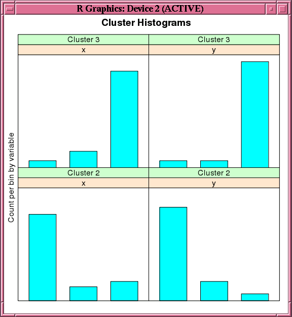
Description of "Figure 4-4 Output of the histogram Function for the ore.odmOC Model"
Building a Support Vector Machine Model
The ore.odmSVM function builds an Oracle Data Mining Support Vector Machine (SVM) model. SVM is a powerful, state-of-the-art algorithm with strong theoretical foundations based on the Vapnik-Chervonenkis theory. SVM has strong regularization properties. Regularization refers to the generalization of the model to new data.
SVM models have similar functional form to neural networks and radial basis functions, both popular data mining techniques.
SVM can be used to solve the following problems:
-
Classification: SVM classification is based on decision planes that define decision boundaries. A decision plane is one that separates between a set of objects having different class memberships. SVM finds the vectors (”support vectors”) that define the separators that give the widest separation of classes.
SVM classification supports both binary and multiclass targets.
-
Regression: SVM uses an epsilon-insensitive loss function to solve regression problems.
SVM regression tries to find a continuous function such that the maximum number of data points lie within the epsilon-wide insensitivity tube. Predictions falling within epsilon distance of the true target value are not interpreted as errors.
-
Anomaly Detection: Anomaly detection identifies identify cases that are unusual within data that is seemingly homogeneous. Anomaly detection is an important tool for detecting fraud, network intrusion, and other rare events that may have great significance but are hard to find.
Anomaly detection is implemented as one-class SVM classification. An anomaly detection model predicts whether a data point is typical for a given distribution or not.
The ore.odmSVM function builds each of these three different types of models. Some arguments apply to classification models only, some to regression models only, and some to anomaly detection models only.
For information on the ore.odmSVM function arguments, invoke help(ore.odmSVM).
Example 4-18 demonstrates the use of SVM classification. The example creates mtcars in the database from the R mtcars data set, builds a classification model, makes predictions, and finally generates a confusion matrix.
Example 4-18 Using the ore.odmSVM Function and Generating a Confusion Matrix
m <- mtcars
m$gear <- as.factor(m$gear)
m$cyl  <- as.factor(m$cyl)
m$vs   <- as.factor(m$vs)
m$ID   <- 1:nrow(m)
mtcars_of <- ore.push(m)
svm.mod  <- ore.odmSVM(gear ~ .-ID, mtcars_of, "classification")
summary(svm.mod)
svm.res  <- predict (svm.mod, mtcars_of,"gear")
with(svm.res, table(gear, PREDICTION))  # generate confusion matrix
Listing for Example 4-18
R> m <- mtcars
R> m$gear <- as.factor(m$gear)
R> m$cyl  <- as.factor(m$cyl)
R> m$vs   <- as.factor(m$vs)
R> m$ID   <- 1:nrow(m)
R> mtcars_of <- ore.push(m)
R>
R> svm.mod  <- ore.odmSVM(gear ~ .-ID, mtcars_of, "classification")
R> summary(svm.mod)
Call:
ore.odmSVM(formula = gear ~ . - ID, data = mtcars_of, type = "classification")

Settings:
                      value
prep.auto                on
active.learning   al.enable
complexity.factor  0.385498
conv.tolerance        1e-04
kernel.cache.size  50000000
kernel.function    gaussian
std.dev            1.072341

Coefficients:
[1] No coefficients with gaussian kernel
R> svm.res  <- predict (svm.mod, mtcars_of,"gear")
R> with(svm.res, table(gear, PREDICTION))  # generate confusion matrix
    PREDICTION
gear  3  4
   3 12  3
   4  0 12
   5  2  3
Example 4-19 demonstrates SVM regression. The example creates a data frame, pushes it to a table, and then builds a regression model; note that ore.odmSVM specifies a linear kernel.
Example 4-19 Using the ore.odmSVM Function and Building a Regression Model
x <- seq(0.1, 5, by = 0.02)
y <- log(x) + rnorm(x, sd = 0.2)
dat <-ore.push(data.frame(x=x, y=y))

# Build model with linear kernel
svm.mod <- ore.odmSVM(y~x,dat,"regression", kernel.function="linear")
summary(svm.mod)
coef(svm.mod)
svm.res <- predict(svm.mod,dat, supplemental.cols="x")
head(svm.res,6)
Listing for Example 4-19
R> x <- seq(0.1, 5, by = 0.02)
R> y <- log(x) + rnorm(x, sd = 0.2)
R> dat <-ore.push(data.frame(x=x, y=y))
R>
R> # Build model with linear kernel
R> svm.mod <- ore.odmSVM(y~x,dat,"regression", kernel.function="linear")
R> summary(svm.mod)

Call:
ore.odmSVM(formula = y ~ x, data = dat, type = "regression",
    kernel.function = "linear")

Settings:
                      value
prep.auto                on
active.learning   al.enable
complexity.factor  0.620553
conv.tolerance        1e-04
epsilon            0.098558
kernel.function      linear

Residuals:
    Min.  1st Qu.   Median     Mean  3rd Qu.     Max.
-0.79130 -0.28210 -0.05592 -0.01420  0.21460  1.58400

Coefficients:
     variable value  estimate
1           x       0.6637951
2 (Intercept)       0.3802170

R> coef(svm.mod)
     variable value  estimate
1           x       0.6637951
2 (Intercept)       0.3802170
R> svm.res <- predict(svm.mod,dat, supplemental.cols="x")
R> head(svm.res,6)
     x PREDICTION
1 0.10 -0.7384312
2 0.12 -0.7271410
3 0.14 -0.7158507
4 0.16 -0.7045604
5 0.18 -0.6932702
6 0.20 -0.6819799
This example of SVN anomaly detection uses mtcars_of created in the classification example and builds an anomaly detection model.
Example 4-20 Using the ore.odmSVM Function and Building an Anomaly Detection Model
svm.mod  <- ore.odmSVM(~ .-ID, mtcars_of, "anomaly.detection")
summary(svm.mod)
svm.res  <- predict (svm.mod, mtcars_of, "ID")
head(svm.res)
table(svm.res$PREDICTION)
Listing for Example 4-18
R> svm.mod  <- ore.odmSVM(~ .-ID, mtcars_of, "anomaly.detection")
R> summary(svm.mod)

Call:
ore.odmSVM(formula = ~. - ID, data = mtcars_of, type = "anomaly.detection")

Settings:
                      value
prep.auto                on
active.learning   al.enable
conv.tolerance        1e-04
kernel.cache.size  50000000
kernel.function    gaussian
outlier.rate             .1
std.dev            0.719126

Coefficients:
[1] No coefficients with gaussian kernel

R> svm.res  <- predict (svm.mod, mtcars_of, "ID")
R> head(svm.res)
                        '0'       '1' ID PREDICTION
Mazda RX4         0.4999405 0.5000595  1          1
Mazda RX4 Wag     0.4999794 0.5000206  2          1
Datsun 710        0.4999618 0.5000382  3          1
Hornet 4 Drive    0.4999819 0.5000181  4          1
Hornet Sportabout 0.4949872 0.5050128  5          1
Valiant           0.4999415 0.5000585  6          1
R> table(svm.res$PREDICTION)

 0  1
 5 27
Cross-Validating Models
Predictive models are usually built on given data and verified on held-aside or unseen data. Cross-validation is a model improvement technique that avoids the limitations of a single train-and-test experiment by building and testing multiple models through repeated sampling from the available data. It's purpose is to offer better insight into how well the model would generalize to new data and to avoid over-fitting and deriving wrong conclusions from misleading peculiarities of the seen data.
The ore.CV utility R function uses Oracle R Enterprise for performing cross-validation of regression and classification models. The function ore.CV is available for download from the following Oracle R Technologies blog post:
https://blogs.oracle.com/R/entry/model_cross_validation_with_ore
For a select set of algorithms and cases, the function ore.CV performs cross-validation for models that were generated by Oracle R Enterprise regression and classification functions using in-database data.
The ore.CV function works with models generated by the following Oracle R Enterprise functions:
-
ore.lm -
ore.stepwise -
ore.glm -
ore.neural -
ore.odmDT -
ore.odmGLM -
ore.odmNB -
ore.odmSVM
You can also use ore.CV to cross-validate models generated with some R regression functions through Oracle R Enterprise embedded R execution. Those R functions are the following:
-
lm
-
glm -
svm
For more information on, and examples of, using ore.CV, and to download the function itself, see the blog post.