3 Preparing and Exploring Data in the Database
This chapter describes how to use Oracle R Enterprise objects to prepare data for analysis and to perform exploratory analysis of the data. All of these functions make it easier for you to prepare very large enterprise database-resident data for modeling. The chapter contains the following topics:
Preparing Data in the Database Using Oracle R Enterprise
Using Oracle R Enterprise, you can prepare data for analysis in the database, as described in the following topics:
About Preparing Data in the Database
Oracle R Enterprise provides functions that enable you to use R to prepare database data for analysis. Using these functions, you can perform typical data preparation tasks on ore.frame and other Oracle R Enterprise objects. You can perform data preparation operations on large quantities of data in the database and then pull the results to your local R session for analysis using functions in packages available from The Comprehensive R Archive Network (CRAN).
You can do operations on data such as the following.
-
Selecting
-
Binning
-
Sampling
-
Sorting and Ordering
-
Summarizing
-
Transforming
-
Performing data preparation operations on date and time data
Performing these operations is described in the other topics in this chapter.
Selecting Data
A typical step in preparing data for analysis is selecting or filtering values of interest from a larger data set. The examples in this section demonstrate selecting data from an ore.frame object by column, by row, and by value. The examples are in the following topics:
See Also:
-
The
sql_like.Rexample script
Selecting Data by Column
Example 3-1 selects columns from an ore.frame object. It first creates a temporary database table, with the corresponding proxy ore.frame object iris_of, from the iris data.frame object. It displays the first three rows of iris_of. The example selects two columns from iris_of and creates the ore.frame object iris_projected with them. It then displays the first three rows of iris_projected.
Example 3-1 Selecting Data by Column
iris_of <- ore.push(iris)
head(iris_of, 3)

iris_projected = iris_of[, c("Petal.Length", "Species")]

head (iris_projected, 3)
Listing for Example 3-1
iris_of <- ore.push(iris)
head(iris_of, 3)
  Sepal.Length Sepal.Width Petal.Length Petal.Width Species
1          5.1         3.5          1.4         0.2  setosa
2          4.9         3.0          1.4         0.2  setosa
3          4.7         3.2          1.3         0.2  setosa

R> iris_projected = iris_of[, c("Petal.Length", "Species")]

R> head (iris_projected, 3)
  Petal.Length Species
1          1.4  setosa
2          1.4  setosa
3          1.3  setosa
Selecting Data by Row
Example 3-2 selects rows from an ordered ore.frame object. The example first adds a column to the iris data.frame object for use in creating an ordered ore.frame object. It invokes the ore.drop function to delete the database table IRIS_TABLE, if it exists. It then creates a database table, with the corresponding proxy ore.frame object IRIS_TABLE, from the iris data.frame. The example invokes the ore.exec function to execute a SQL statement that makes the RID column the primary key of the database table. It then invokes the ore.sync function to synchronize the IRIS_TABLE ore.frame object with the table and displays the first three rows of the proxy ore.frame object.
Example 3-2 next selects 51 rows from IRIS_TABLE by row number and creates the ordered ore.frame object iris_selrows with them. It displays the first six rows of iris_selrows. It then selects 3 rows by row name and displays the result.
Example 3-2 Selecting Data by Row
# Add a column to the iris data set to use as row identifiers.
iris$RID <- as.integer(1:nrow(iris) + 100)
ore.drop(table = 'IRIS_TABLE')
ore.create(iris, table = 'IRIS_TABLE')
ore.exec("alter table IRIS_TABLE add constraint IRIS_TABLE
          primary key (\"RID\")")
ore.sync(table = "IRIS_TABLE")
head(IRIS_TABLE, 3)

# Select rows by row number.
iris_selrows <- IRIS_TABLE[50:100,]
head(iris_selrows)

# Select rows by row name.
IRIS_TABLE[c("101", "151", "201"),]
Listing for Example 3-2
R> # Add a column to the iris data set to use as row identifiers.
R> iris$RID <- as.integer(1:nrow(iris) + 100)
R> ore.drop(table = 'IRIS_TABLE')
R> ore.create(iris, table = 'IRIS_TABLE')
R> ore.exec("alter table IRIS_TABLE add constraint IRIS_TABLE
+            primary key (\"RID\")")
R> ore.sync(table = "IRIS_TABLE")
R> head(IRIS_TABLE, 3)
    Sepal.Length Sepal.Width Petal.Length Petal.Width Species RID
101          5.1         3.5          1.4         0.2  setosa 101
102          4.9         3.0          1.4         0.2  setosa 102
103          4.7         3.2          1.3         0.2  setosa 103
R> # Select rows by row number.
R> iris_selrows <- IRIS_TABLE[50:100,]
R> head(iris_selrows)
    Sepal.Length Sepal.Width Petal.Length Petal.Width    Species RID
150          5.0         3.3          1.4         0.2     setosa 150
151          7.0         3.2          4.7         1.4 versicolor 151
152          6.4         3.2          4.5         1.5 versicolor 152
153          6.9         3.1          4.9         1.5 versicolor 153
154          5.5         2.3          4.0         1.3 versicolor 154
155          6.5         2.8          4.6         1.5 versicolor 155
R> # Select rows by row name.
R> IRIS_TABLE[c("101", "151", "201"),]
    Sepal.Length Sepal.Width Petal.Length Petal.Width    Species RID
101          5.1         3.5          1.4         0.2     setosa 101
151          7.0         3.2          4.7         1.4 versicolor 151
201          6.3         3.3          6.0         2.5  virginica 201
Selecting Data by Value
You can select portions of a data set, as shown in Example 3-3. The example pushes the iris data set to the database and gets the ore.frame object iris_of. It filters the data to produce iris_of_filtered, which contains the values from the rows of iris_of that have a petal length of less than 1.5 and that are in the Sepal.Length and Species columns. The example also filters the data using conditions, so that iris_of_filtered contains the values from iris_of that are of the setosa or versicolor species and that have a petal width of less than 2.0.
Example 3-3 Selecting Data by Value
iris_of <- ore.push(iris)
# Select sepal length and species where petal length is less than 1.5.
iris_of_filtered <- iris_of[iris_of$Petal.Length < 1.5,
                            c("Sepal.Length", "Species")]
names(iris_of_filtered)
nrow(iris_of_filtered)
head(iris_of_filtered, 3)
# Alternate syntax filtering.
iris_of_filtered <- subset(iris_of, Petal.Length < 1.5)
nrow(iris_of_filtered)
head(iris_of_filtered, 3)
# Using the AND and OR conditions in filtering.
# Select all rows with in which the species is setosa or versicolor.
# and the petal width is less than 2.0.
iris_of_filtered <- iris_of[(iris_of$Species == "setosa" |
                             iris_of$Species == "versicolor") &
                             iris_of$Petal.Width < 2.0,]
nrow(iris_of_filtered)
head(iris_of, 3)
Listing for Example 3-3
R> iris_of <- ore.push(iris)
R> # Select sepal length and species where petal length is less than 1.5.
R> iris_of_filtered <- iris_of[iris_of$Petal.Length < 1.5,
+                              c("Sepal.Length", "Species")]
R> names(iris_of_filtered)
[1] "Sepal.Length" "Species"
R> nrow(iris_of_filtered)
[1] 24
R> head(iris_of_filtered, 3)
  Sepal.Length Species
1          5.1  setosa
2          4.9  setosa
3          4.7  setosa
R> # Alternate syntax filtering.
R> iris_of_filtered <- subset(iris_of, Petal.Length < 1.5)
R> nrow(iris_of_filtered)[1] 24
R> head(iris_of_filtered, 3)
  Sepal.Length Sepal.Width Petal.Length Petal.Width Species
1          5.1         3.5          1.4         0.2  setosa
2          4.9         3.0          1.4         0.2  setosa
3          4.7         3.2          1.3         0.2  setosa
R> # Using the AND and OR conditions in filtering.
R> # Select all rows with in which the species is setosa or versicolor.
R> # and the petal width is less than 2.0.
R> iris_of_filtered <- iris_of[(iris_of$Species == "setosa" |
+                              iris_of$Species == "versicolor") &
+                              iris_of$Petal.Width < 2.0,]
R> nrow(iris_of_filtered)[1] 100
R> head(iris_of, 3)
  Sepal.Length Sepal.Width Petal.Length Petal.Width Species
1          5.1         3.5          1.4         0.2  setosa
2          4.9         3.0          1.4         0.2  setosa
3          4.7         3.2          1.3         0.2  setosa
Indexing Data
You can use integer or character vectors to index an ordered ore.frame object. You can use the indexing to perform sampling and partitioning, as described in "Sampling Data" and "Partitioning Data".
Oracle R Enterprise supports functionality similar to R indexing with these differences:
-
Integer indexing is not supported for
ore.vectorobjects. -
Negative integer indexes are not supported.
-
Row order is not preserved.
Example 3-4 demonstrates character and integer indexing. The example uses the ordered SPAM_PK and unordered SPAM_NOPK ore.frame objects from Example 2-13. The example shows that you can access rows by name and that you can also access a set of rows by supplying a vector of character row names. The example then shows that you can supply the actual integer value. In the example this results in a set of different rows because the USERID values start at 1001, as opposed to 1.
Example 3-4 Indexing an ore.frame Object
# Index to a specifically named row.
SPAM_PK["2060", 1:4]
# Index to a range of rows by row names.
SPAM_PK[as.character(2060:2064), 1:4]
# Index to a range of rows by integer index.
SPAM_PK[2060:2063, 1:4]
Listing for Example 3-4
R> # Index to a specifically named row.
R> SPAM_PK["2060", 1:4]
       TS USERID make address
2060 2060    380    0       0
R> # Index to a range of rows by row names.
R> SPAM_PK[as.character(2060:2064), 1:4]
       TS USERID make address
2060 2060    380    0       0
2061 2061    381    0       0
2062 2062    381    0       0
2063 2063    382    0       0
2064 2064    382    0       0
R> # Index to a range of rows by integer index.
R> SPAM_PK[2060:2063, 1:4]
       TS USERID make address
3060 3060    380 0.00    0.00
3061 3061    381 0.00    1.32
3062 3062    381 0.00    2.07
3063 3063    382 0.34    0.00
Combining Data
You can join data from ore.frame objects that represent database tables by using the merge function, as shown in Example 3-5. The example creates two data.frame objects and merges them. It then invokes the ore.create function to create a database table for each data.frame object. The ore.create function automatically generates an ore.frame object as a proxy object for the table. The ore.frame object has the same name as the table. The example merges the ore.frame objects. Note that the order of the results of the two merge operations is not the same because the ore.frame objects are unordered.
Example 3-5 Joining Data from Two Tables
# Create data.frame objects.
df1 <- data.frame(x1=1:5, y1=letters[1:5])
df2 <- data.frame(x2=5:1, y2=letters[11:15])

# Combine the data.frame objects.
merge (df1, df2, by.x="x1", by.y="x2")

# Create database tables and ore.frame proxy objects to correspond to
# the local R objects df1 and df2.
ore.create(df1, table="DF1_TABLE")
ore.create(df2, table="DF2_TABLE")

# Combine the ore.frame objects.
merge (DF1_TABLE, DF2_TABLE, by.x="x1", by.y="x2")
Listing for Example 3-5
R> # Create data.frame objects.
R> df1 <- data.frame(x1=1:5, y1=letters[1:5])
R> df2 <- data.frame(x2=5:1, y2=letters[11:15])

R> # Combine the data.frame objects.
R> merge (df1, df2, by.x="x1", by.y="x2")
  x1 y1 y2
1  1  a  o
2  2  b  n
3  3  c  m
4  4  d  l
5  5  e  k

R> # Create database tables and ore.frame proxy objects to correspond to
R> # the local R objects df1 and df2.
R> ore.create(df1, table="DF1_TABLE")
R> ore.create(df2, table="DF2_TABLE")

R> # Combine the ore.frame objects.
R> merge (DF1_TABLE, DF2_TABLE, by.x="x1", by.y="x2")
  x1 y1 y2
1  5  e  k
2  4  d  l
3  3  c  m
4  2  b  n
5  1  a  o
Warning message:
ORE object has no unique key - using random order
Summarizing Data
You can summarize data by using the aggregate function, as shown in Example 3-6. The example pushes the iris data set to database memory as the ore.frame object iris_of. It aggregates the values of iris_of by the Species column using the length function. It then displays the first three rows of the result.
# Create a temporary database table from the iris data set and get an ore.frame.
iris_of <- ore.push(iris)
aggdata <- aggregate(iris_of$Sepal.Length,
                     by = list(species = iris_of$Species),
                     FUN = length)
head(aggdata, 3)
Listing for Example 3-6
# Create a temporary database table from the iris data set and get an ore.frame.
R> iris_of <- ore.push(iris)
R> aggdata <- aggregate(iris_of$Sepal.Length,
+                      by = list(species = iris_of$Species),
+                      FUN = length)
R> head(aggdata, 3)
             species  x
setosa         setosa 50
versicolor versicolor 50
virginica   virginica 50
See Also:
Theaggregate.R example scriptTransforming Data
In preparing data for analysis, a typical step is to transform data by reformatting it or deriving new columns and adding them to the data set. The examples in this topic demonstrate two ways of formatting data and deriving columns. Example 3-7 creates a function to format the data in a column and Example 3-8 does the same thing by using the transform function. Example 3-9 uses the transform function to add columns to the data set.
# Create a function for formatting data.
petalCategory_fmt <- function(x) {
    ifelse(x > 5, 'LONG',
    ifelse(x > 2, 'MEDIUM', 'SMALL'))
  }
# Create an ore.frame in database memory with the iris data set.
iris_of <- ore.push(iris)
# Select some rows from iris_of.
iris_of[c(10, 20, 60, 80, 110, 140),]
# Format the data in Petal.Length column.
iris_of$Petal.Length <- petalCategory_fmt(iris_of$Petal.Length)
# Select the same rows from iris_of.
Listing for Example 3-7
R> # Create a function for formatting data.
R> petalCategory_fmt <- function(x) {
+    ifelse(x > 5, 'LONG',
+    ifelse(x > 2, 'MEDIUM', 'SMALL'))
+ }
R> # Create an ore.frame in database memory with the iris data set.
R> iris_of <- ore.push(iris)
R> # Select some rows from iris_of.
R> iris_of[c(10, 20, 60, 80, 110, 140),]
    Sepal.Length Sepal.Width Petal.Length Petal.Width    Species
10           4.9         3.1          1.5         0.1     setosa
20           5.1         3.8          1.5         0.3     setosa
60           5.2         2.7          3.9         1.4 versicolor
80           5.7         2.6          3.5         1.0 versicolor
110          7.2         3.6          6.1         2.5  virginica
140          6.9         3.1          5.4         2.1  virginica
R> # Format the data in Petal.Length column.
R> iris_of$Petal.Length <- petalCategory_fmt(iris_of$Petal.Length)
# Select the same rows from iris_of.
R> iris_of[c(10, 20, 60, 80, 110, 140),]
    Sepal.Length Sepal.Width Petal.Length Petal.Width    Species
10           4.9         3.1        SMALL         0.1     setosa
20           5.1         3.8        SMALL         0.3     setosa
60           5.2         2.7       MEDIUM         1.4 versicolor
80           5.7         2.6       MEDIUM         1.0 versicolor
110          7.2         3.6         LONG         2.5  virginica
140          6.9         3.1         LONG         2.1  virginica
Example 3-8 does the same thing as Example 3-7 except that it uses the transform function to reformat the data in a column of the data set.
Example 3-8 Using the transform Function
# Create an ore.frame in database memory with the iris data set.
iris_of2 <- ore.push(iris)
# Select some rows from iris_of.
iris_of2[c(10, 20, 60, 80, 110, 140),]
iris_of2 <- transform(iris_of2,
                  Petal.Length = ifelse(Petal.Length > 5, 'LONG',
                                 ifelse(Petal.Length > 2, 'MEDIUM', 'SMALL')))
iris_of2[c(10, 20, 60, 80, 110, 140),]
Listing for Example 3-8
R> # Create an ore.frame in database memory with the iris data set.
R> iris_of2 <- ore.push(iris)
R> # Select some rows from iris_of.
R> iris_of2[c(10, 20, 60, 80, 110, 140),]
    Sepal.Length Sepal.Width Petal.Length Petal.Width    Species
10           4.9         3.1          1.5         0.1     setosa
20           5.1         3.8          1.5         0.3     setosa
60           5.2         2.7          3.9         1.4 versicolor
80           5.7         2.6          3.5         1.0 versicolor
110          7.2         3.6          6.1         2.5  virginica
140          6.9         3.1          5.4         2.1  virginica
R> iris_of2 <- transform(iris_of2,
+                  Petal.Length = ifelse(Petal.Length > 5, 'LONG',
+                                 ifelse(Petal.Length > 2, 'MEDIUM', 'SMALL')))
R> iris_of2[c(10, 20, 60, 80, 110, 140),]
    Sepal.Length Sepal.Width Petal.Length Petal.Width    Species
10           4.9         3.1        SMALL         0.1     setosa
20           5.1         3.8        SMALL         0.3     setosa
60           5.2         2.7       MEDIUM         1.4 versicolor
80           5.7         2.6       MEDIUM         1.0 versicolor
110          7.2         3.6         LONG         2.5  virginica
140          6.9         3.1         LONG         2.1  virginica
Example 3-9 uses the transform function to add a derived column to the data set and then to add additional columns to it.
Example 3-9 Adding Derived Columns
# Set the page width.
options(width = 80)
# Create an ore.frame in database memory with the iris data set.
iris_of <- ore.push(iris)
names(iris_of)
# Add one column derived from another
iris_of <- transform(iris_of, LOG_PL = log(Petal.Length))
names(iris_of)
head(iris_of, 3)
# Add more columns.
iris_of <- transform(iris_of,
                    SEPALBINS = ifelse(Sepal.Length < 6.0, "A", "B"),
                    PRODUCTCOLUMN = Petal.Length * Petal.Width,
                    CONSTANTCOLUMN = 10)
names(iris_of)
# Select some rows of iris_of.
iris_of[c(10, 20, 60, 80, 110, 140),]
Listing for Example 3-9
R> # Set the page width.
R> options(width = 80)
R> # Create an ore.frame in database memory with the iris data set.
R> iris_of <- ore.push(iris)
R> names(iris_of)
[1] "Sepal.Length" "Sepal.Width"  "Petal.Length" "Petal.Width"  "Species"
R> # Add one column derived from another
R> iris_of <- transform(iris_of, LOG_PL = log(Petal.Length))
R> names(iris_of)
[1] "Sepal.Length" "Sepal.Width"  "Petal.Length" "Petal.Width"  "Species"
[6] "LOG_PL"
R> head(iris_of, 3)
  Sepal.Length Sepal.Width Petal.Length Petal.Width Species    LOG_PL
1          5.1         3.5          1.4         0.2  setosa 0.3364722
2          4.9         3.0          1.4         0.2  setosa 0.3364722
3          4.7         3.2          1.3         0.2  setosa 0.2623643
R> # Add more columns.
R> iris_of <- transform(iris_of,
                    SEPALBINS = ifelse(Sepal.Length < 6.0, "A", "B"),
                    PRODUCTCOLUMN = Petal.Length * Petal.Width,
                    CONSTANTCOLUMN = 10)
R> names(iris_of)
[1] "Sepal.Length"   "Sepal.Width"    "Petal.Length"   "Petal.Width"
[5] "Species"        "LOG_PL"         "CONSTANTCOLUMN" "SEPALBINS"
[9] "PRODUCTCOLUMN"
R> # Select some rows of iris_of.
R> iris_of[c(10, 20, 60, 80, 110, 140),]
    Sepal.Length Sepal.Width Petal.Length Petal.Width    Species    LOG_PL
10           4.9         3.1          1.5         0.1     setosa 0.4054651
20           5.1         3.8          1.5         0.3     setosa 0.4054651
60           5.2         2.7          3.9         1.4 versicolor 1.3609766
80           5.7         2.6          3.5         1.0 versicolor 1.2527630
110          7.2         3.6          6.1         2.5  virginica 1.8082888
140          6.9         3.1          5.4         2.1  virginica 1.6863990
    CONSTANTCOLUMN SEPALBINS PRODUCTCOLUMN
10              10         A          0.15
20              10         A          0.45
60              10         A          5.46
80              10         A          3.50
110             10         B         15.25
140             10         B         11.34
See Also:
Thederived.R example scriptSampling Data
Sampling is an important capability for statistical analytics. Typically, you sample data to reduce its size and to perform meaningful work on it. In R you usually must load data into memory to sample it. However, if the data is too large, this isn't possible.
In Oracle R Enterprise, instead of pulling the data from the database and then sampling, you can sample directly in the database and then pull only those records that are part of the sample. By sampling in the database, you minimize data movement and you can work with larger data sets. Note that it is the ordering framework integer row indexing in the transparency layer that enables this capability.
Note:
Sampling requires using ordered ore.frame objects as described in "Creating Ordered and Unordered ore.frame Objects".The examples in this section illustrate several sampling techniques. Similar examples are in the sampling.R example script.
Example 3-10 demonstrates a simple selection of rows at random. The example creates a small data.frame object and pushes it to the database to create an ore.frame object, MYDATA. Out of 20 rows, the example samples 5. It uses the R sample function to produce a random set of indices that it uses to get the sample from MYDATA. The sample, simpleRandomSample, is an ore.frame object.
Example 3-10 Simple Random Sampling
set.seed(1)
N <- 20
myData <- data.frame(a=1:N,b=letters[1:N])
MYDATA <- ore.push(myData)
head(MYDATA)
sampleSize <- 5
simpleRandomSample <- MYDATA[sample(nrow(MYDATA), sampleSize), , drop=FALSE]
class(simpleRandomSample)
simpleRandomSample
Listing for Example 3-10
R> set.seed(1)
R> N <- 20
R> myData <- data.frame(a=1:N,b=letters[1:N])
R> MYDATA <- ore.push(myData)
R> head(MYDATA)
  a b
1 1 a
2 2 b
3 3 c
4 4 d
5 5 e
6 6 f
R> sampleSize <- 5
R> simpleRandomSample <- MYDATA[sample(nrow(MYDATA), sampleSize), , drop=FALSE]
R> class(simpleRandomSample)
[1] "ore.frame"
attr(,"package")
[1] "OREbase"
R> simpleRandomSample
    a b
2   2 b
7   7 g
10 10 j
12 12 l
19 19 s
Example 3-11 demonstrates randomly partitioning data into training and testing sets. This splitting of the data is normally done in classification and regression to assess how well a model performs on new data. The example uses the MYDATA object created in Example 3-10.
Example 3-11 produces a sample set of indices to use as the test data set. It then creates the logical vector group that is TRUE if the index is in the sample and is FALSE otherwise. Next, it uses row indexing to produce the training set where the group is FALSE and the test set where the group is TRUE. Notice that the number of rows in the training set is 15 and the number of rows in the test set is 5, as specified in the invocation of the sample function.
Example 3-11 Split Data Sampling
set.seed(1)
sampleSize <- 5
ind <- sample(1:nrow(MYDATA), sampleSize)
group <- as.integer(1:nrow(MYDATA) %in% ind)
MYDATA.train <- MYDATA[group==FALSE,]
dim(MYDATA.train)
MYDATA.test <- MYDATA[group==TRUE,]
dim(MYDATA.test)
Listing for Example 3-11
R> set.seed(1)
R> sampleSize <- 5
R> ind <- sample(1:nrow(MYDATA), sampleSize)
R> group <- as.integer(1:nrow(MYDATA) %in% ind)
R> MYDATA.train <- MYDATA[group==FALSE,]
dim(MYDATA.train)
[1] 15  2
R> MYDATA.test <- MYDATA[group==TRUE,]
R> dim(MYDATA.test)
[1] 5 2
Example 3-12 demonstrates systematic sampling, in which rows are selected at regular intervals. The example uses the seq function to create a sequence of values that start at 2 and increase by increments of 3. The number of values in the sequence is equal to the number of rows in MYDATA. The MYDATA object is created in Example 3-10.
Example 3-12 Systematic Sampling
set.seed(1)
N <- 20
myData <- data.frame(a=1:20,b=letters[1:N])
MYDATA <- ore.push(myData)
head(MYDATA)
start <- 2
by <- 3
systematicSample <- MYDATA[seq(start, nrow(MYDATA), by = by), , drop = FALSE]
systematicSample
Listing for Example 3-12
R> set.seed(1)
R> N <- 20
R> myData <- data.frame(a=1:20,b=letters[1:N])
R> MYDATA <- ore.push(myData)
R> head(MYDATA)
  a b
1 1 a
2 2 b
3 3 c
4 4 d
5 5 e
6 6 f
R> start <- 2
R> by <- 3
R> systematicSample <- MYDATA[seq(start, nrow(MYDATA), by = by), , drop = FALSE]
systematicSample
    a b
2   2 b
5   5 e
8   8 h
11 11 k
14 14 n
17 17 q
20 20 t
Example 3-13 demonstrates stratified sampling, in which rows are selected within each group where the group is determined by the values of a particular column. The example creates a data set that has each row assigned to a group. The function rnorm produces random normal numbers. The argument 4 is the desired mean for the distribution. The example splits the data according to group and then samples proportionately from each partition. Finally, it row binds the list of subset ore.frame objects into a single ore.frame object and then displays the values of the result, stratifiedSample.
Example 3-13 Stratified Sampling
set.seed(1)
N <- 200
myData <- data.frame(a=1:N,b=round(rnorm(N),2),
                     group=round(rnorm(N,4),0))
MYDATA <- ore.push(myData)
head(MYDATA)
sampleSize <- 10
stratifiedSample <- do.call(rbind,
                            lapply(split(MYDATA, MYDATA$group),
                                   function(y) {
                                   ny <- nrow(y)
                                   y[sample(ny, sampleSize*ny/N), , drop = FALSE]
                              }))
stratifiedSample
Listing for Example 3-13
R> set.seed(1)
R> N <- 200
R> myData <- data.frame(a=1:N,b=round(rnorm(N),2),
+                       group=round(rnorm(N,4),0))
R> MYDATA <- ore.push(myData)
R> head(MYDATA)
  a     b group
1 1 -0.63     4
2 2  0.18     6
3 3 -0.84     6
4 4  1.60     4
5 5  0.33     2
6 6 -0.82     6
R> sampleSize <- 10
R> stratifiedSample <- do.call(rbind,
+                              lapply(split(MYDATA, MYDATA$group),
+                                function(y) {
+                                  ny <- nrow(y)
+                                  y[sample(ny, sampleSize*ny/N), , drop = FALSE]
+                             }))
R> stratifiedSample
          a     b group
173|173 173  0.46     3
9|9       9  0.58     4
53|53    53  0.34     4
139|139 139 -0.65     4
188|188 188 -0.77     4
78|78    78  0.00     5
137|137 137 -0.30     5
Example 3-14 demonstrates cluster sampling, in which entire groups are selected at random. The example splits the data according to group and then samples among the groups and row binds into a single ore.frame object. The resulting sample has data from two clusters, 6 and 7.
set.seed(1)
N <- 200
myData <- data.frame(a=1:N,b=round(runif(N),2),
                     group=round(rnorm(N,4),0))
MYDATA <- ore.push(myData)
head(MYDATA)
sampleSize <- 5
clusterSample <- do.call(rbind,
                         sample(split(MYDATA, MYDATA$group), 2))
unique(clusterSample$group)
Listing for Example 3-14
R> set.seed(1)
R> N <- 200
R> myData <- data.frame(a=1:N,b=round(runif(N),2),
+                       group=round(rnorm(N,4),0))
R> MYDATA <- ore.push(myData)
R> head(MYDATA)
  a    b group
1 1 0.27     3
2 2 0.37     4
3 3 0.57     3
4 4 0.91     4
5 5 0.20     3
6 6 0.90     6
R> sampleSize <- 5
R> clusterSample <- do.call(rbind,
+                           sample(split(MYDATA, MYDATA$group), 2))
R> unique(clusterSample$group)
[1] 6 7
Example 3-15 demonstrates quota sampling, in which a consecutive number of records are selected as the sample. The example uses the head function to select the sample. The tail function could also have been used.
set.seed(1)
N <- 200
myData <- data.frame(a=1:N,b=round(runif(N),2))
MYDATA <- ore.push(myData)
sampleSize <- 10
quotaSample1 <- head(MYDATA, sampleSize)
quotaSample1
Listing for Example 3-15
R> set.seed(1)
R> N <- 200
R> myData <- data.frame(a=1:N,b=round(runif(N),2))
R> MYDATA <- ore.push(myData)
R> sampleSize <- 10
R> quotaSample1 <- head(MYDATA, sampleSize)
R> quotaSample1
    a    b
1   1 0.15
2   2 0.75
3   3 0.98
4   4 0.97
5   5 0.35
6   6 0.39
7   7 0.95
8   8 0.11
9   9 0.93
10 10 0.35
Partitioning Data
In analyzing large data sets, a typical operation is to randomly partitioning the data set into subsets. You can analyze the partitions by using Oracle R Enterprise embedded R execution, as shown in Example 3-16. The example creates a data.frame object with the symbol myData in the local R session and adds a column to it that contains a randomly generated set of values. It pushes the data set to database memory as the object MYDATA. The example invokes the embedded R execution function ore.groupApply, which partitions the data based on the partition column and then applies the lm function to each partition.
Example 3-16 Randomly Partitioning Data
N <- 200
k <- 5
myData <- data.frame(a=1:N,b=round(runif(N),2))
myData$partition <- sample(rep(1:k, each = N/k,
                               length.out = N), replace = TRUE)
MYDATA <- ore.push(myData)
head(MYDATA)
results <- ore.groupApply(MYDATA, MYDATA$partition,
                          function(y) {lm(b~a,y)}, parallel = TRUE)
length(results)
results[[1]]
Listing for Example 3-16
R> N <- 200
R> k <- 5
R> myData <- data.frame(a=1:N,b=round(runif(N),2))
R> myData$partition <- sample(rep(1:k, each = N/k,
+                             length.out = N), replace = TRUE)
R> MYDATA <- ore.push(myData)
R> head(MYDATA)
  a    b partition
1 1 0.89         2
2 2 0.31         4
3 3 0.39         5
4 4 0.66         3
5 5 0.01         1
6 6 0.12         4
R> results <- ore.groupApply(MYDATA, MYDATA$partition,
+                            function(y) {lm(b~a,y)}, parallel = TRUE)
R> length(results)
[1] 5
R> results[[1]]

Call:
lm(formula = b ~ a, data = y)

Coefficients:
(Intercept)            a
   0.388795     0.001015
Preparing Time Series Data
Oracle R Enterprise provides you with the ability to perform many data preparation operations on time series data, such as filtering, ordering, and transforming the data. Oracle R Enterprise maps R data types to SQL data types, as shown in Table 1-1, which allows you to create Oracle R Enterprise objects and perform data preparation operations in database memory.
The following examples demonstrate some operations on time series data.
Example 3-17 illustrates some of the statistical aggregation functions. For a data set, the example first generates on the local client a sequence of five hundred dates spread evenly throughout 2001. It then introduces a random difftime and a vector of random normal values. The example then uses the ore.push function to create MYDATA, an in-database version of the data. The example invokes the class function to show that MYDATA is an ore.frame object and that the datetime column is of class ore.datetime. The example displays the first three rows of the generated data. It then uses the statistical aggregation operations of min, max, range, median, and quantile on the datetime column of MYDATA.
Example 3-17 Aggregating Date and Time Data
N <- 500
mydata <- data.frame(datetime =
                seq(as.POSIXct("2001/01/01"),
                    as.POSIXct("2001/12/31"),
                    length.out = N),
                difftime = as.difftime(runif(N),
                                 units = "mins"),
                x = rnorm(N))
MYDATA <- ore.push(mydata)
class(MYDATA)
class(MYDATA$datetime)
head(MYDATA,3)
# statistical aggregations
min(MYDATA$datetime)
max(MYDATA$datetime)
range(MYDATA$datetime)
quantile(MYDATA$datetime,
         probs = c(0, 0.05, 0.10))
Listing for Example 3-17
R> N <- 500
R> mydata <- data.frame(datetime =
+             seq(as.POSIXct("2001/01/01"),
+                 as.POSIXct("2001/12/31"),
+                 length.out = N),
+             difftime = as.difftime(runif(N),
+                              units = "mins"),
+             x = rnorm(N))
R> MYDATA <- ore.push(mydata)
R> class(MYDATA)
[1] "ore.frame"
attr(,"package")
[1] "OREbase"
R> class(MYDATA$datetime)
[1] "ore.datetime"
attr(,"package")
[1] "OREbase"
R> head(MYDATA,3)
             datetime       difftime           x
1 2001-01-01 00:00:00 16.436782 secs  0.68439244
2 2001-01-01 17:30:25  8.711562 secs  1.38481435
3 2001-01-02 11:00:50  1.366927 secs -0.00927078

R> # statistical aggregations
R> min(MYDATA$datetime)
[1] "2001-01-01 CST"
R> max(MYDATA$datetime)
[1] "2001-12-31 CST"
R> range(MYDATA$datetime)
[1] "2001-01-01 CST" "2001-12-31 CST"
R> quantile(MYDATA$datetime,
+           probs = c(0, 0.05, 0.10))
                       0%                        5%                       10%
"2001-01-01 00:00:00 CST" "2001-01-19 04:48:00 CST" "2001-02-06 09:36:00 CST"
Example 3-18 creates a one day shift by taking the datetime column of the MYDATA ore.frame object created in Example 3-17 and adding a difftime of one day. The result is day1Shift, which the example shows is of class ore.datetime. The example displays the first three elements of the datetime column of MYDATA and those of day1Shift. The first element of day1Shift is January 2, 2001.
Example 3-18 also computes lag differences using the overloaded diff function. The difference between the dates is all the same because the 500 dates in MYDATA are evenly distributed throughout 2001.
Example 3-18 Using Date and Time Arithmetic
day1Shift <- MYDATA$datetime + as.difftime(1, units = "days")
class(day1Shift)
head(MYDATA$datetime,3)
head(day1Shift,3)
lag1Diff <- diff(MYDATA$datetime)
class(lag1Diff)
head(lag1Diff,3)
Listing for Example 3-18
R> day1Shift <- MYDATA$datetime + as.difftime(1, units = "days")
R> class(day1Shift)
[1] "ore.datetime"
attr(,"package")
[1] "OREbase"
R> head(MYDATA$datetime,3)
[1] "2001-01-01 00:00:00 CST" "2001-01-01 17:30:25 CST" "2001-01-02 11:00:50 CST"
R> head(day1Shift,3)
[1] "2001-01-02 00:00:00 CST" "2001-01-02 17:30:25 CST" "2001-01-03 11:00:50 CST"
R> lag1Diff <- diff(MYDATA$datetime)
R> class(lag1Diff)
[1] "ore.difftime"
attr(,"package")
[1] "OREbase"
R> head(lag1Diff,3)
Time differences in secs
[1] 63025.25 63025.25 63025.25
Example 3-19 demonstrates date and time comparisons. The example uses the datetime column of the MYDATA ore.frame object created in Example 3-17. Example 3-19 selects the elements of MYDATA that have a date earlier than April 1, 2001. The resulting isQ1 is of class ore.logical and for the first three entries the result is TRUE. The example finds out how many dates matching isQ1 are in March. It then sums the logical vector and displays the result, which is that 43 rows are in March. The example next filters rows based on dates that are the end of the year, after December 27. The result is eoySubset, which is an ore.frame object. The example displays the first three rows returned in eoySubset.
Example 3-19 Comparing Dates and Times
isQ1 <- MYDATA$datetime < as.Date("2001/04/01")
class(isQ1)
head(isQ1,3)
isMarch <- isQ1 & MYDATA$datetime > as.Date("2001/03/01")
class(isMarch)
head(isMarch,3)
sum(isMarch)
eoySubset <- MYDATA[MYDATA$datetime > as.Date("2001/12/27"), ]
class(eoySubset)
head(eoySubset,3)
Listing for Example 3-19
R> isQ1 <- MYDATA$datetime < as.Date("2001/04/01")
R> class(isQ1)
[1] "ore.logical"
attr(,"package")
[1] "OREbase"
R> head(isQ1,3)
[1] TRUE TRUE TRUE
R> isMarch <- isQ1 & MYDATA$datetime > as.Date("2001/03/01")
R> class(isMarch)
[1] "ore.logical"
attr(,"package")
[1] "OREbase"
R> head(isMarch,3)
[1] FALSE FALSE FALSE
R> sum(isMarch)
[1] 43
R> eoySubset <- MYDATA[MYDATA$datetime > as.Date("2001/12/27"), ]
R> class(eoySubset)
[1] "ore.frame"
attr(,"package")
[1] "OREbase"
R> head(eoySubset,3)
               datetime      difftime          x
495 2001-12-27 08:27:53 55.76474 secs -0.2740492
496 2001-12-28 01:58:18 15.42946 secs -1.4547270
497 2001-12-28 19:28:44 28.62195 secs  0.2929171
Oracle R Enterprise has accessor functions that you can use to extract various components from datetime objects, such as year, month, day of the month, hour, minute, and second. Example 3-20 demonstrates the use of these functions. The example uses the datetime column of the MYDATA ore.frame object created in Example 3-17.
Example 3-20 gets the year elements of the datetime column. The invocation of the unique function for year displays 2001 because it is the only year value in the column. However, for objects that have a range of values, as for example, ore.mday, the range function returns the day of the month. The result contains a vector with values that range from 1 through 31. Invoking the range function succinctly reports the range of values, as demonstrated for the other accessor functions.
Example 3-20 Using Date and Time Accessors
year <- ore.year(MYDATA$datetime)
unique(year)
month <- ore.month(MYDATA$datetime)
range(month)
dayOfMonth <- ore.mday(MYDATA$datetime)
range(dayOfMonth)
hour <- ore.hour(MYDATA$datetime)
range(hour)
minute <- ore.minute(MYDATA$datetime)
range(minute)
second <- ore.second(MYDATA$datetime)
range(second)
Listing for Example 3-20
R> year <- ore.year(MYDATA$datetime)
R> unique(year)
[1] 2001
R> month <- ore.month(MYDATA$datetime)
R> range(month)
[1]  1 12
R> dayOfMonth <- ore.mday(MYDATA$datetime)
R> range(dayOfMonth)
[1]  1 31
R> hour <- ore.hour(MYDATA$datetime)
R> range(hour)
[1]  0 23
R> minute <- ore.minute(MYDATA$datetime)
R> range(minute)
[1]  0 59
R> second <- ore.second(MYDATA$datetime)
R> range(second)
[1]  0.00000 59.87976
Example 3-21 uses the as.ore subclass objects to coerce an ore.datetime data type into other data types. The example uses the datetime column of the MYDATA ore.frame object created in Example 3-17. That column contains ore.datetime values. Example 3-21 first extracts the date from the MYDATA$datetime column. The resulting dateOnly object has ore.date values that contain only the year, month, and day, but not the time. The example then coerces the ore.datetime values into objects with ore.character and ore.integer values that represent the names of days, the number of the day of the year, and the quarter of the year.
Example 3-21 Coercing Date and Time Data Types
dateOnly <- as.ore.date(MYDATA$datetime)
class(dateOnly)
head(sort(unique(dateOnly)),3)
nameOfDay <- as.ore.character(MYDATA$datetime, format = "DAY")
class(nameOfDay)
sort(unique(nameOfDay))
dayOfYear <- as.integer(as.character(MYDATA$datetime, format = "DDD"))
class(dayOfYear)
range(dayOfYear)
quarter <- as.integer(as.character(MYDATA$datetime, format = "Q"))
class(quarter)
sort(unique(quarter))
Listing for Example 3-21
R> dateOnly <- as.ore.date(MYDATA$datetime)
R> class(dateOnly)[1] "ore.date"
attr(,"package")[1] "OREbase"
R> head(sort(unique(dateOnly)),3)
[1] "2001-01-01" "2001-01-02" "2001-01-03"
R> nameOfDay <- as.ore.character(MYDATA$datetime, format = "DAY")
R> class(nameOfDay)
[1] "ore.character"
attr(,"package")
[1] "OREbase"
R> sort(unique(nameOfDay))
[1] "FRIDAY " "MONDAY " "SATURDAY " "SUNDAY " "THURSDAY " "TUESDAY " "WEDNESDAY"
R> dayOfYear <- as.integer(as.character(MYDATA$datetime, format = "DDD"))
R> class(dayOfYear)
[1] "ore.integer"
attr(,"package")
[1] "OREbase"
R> range(dayOfYear)
[1]   1 365
R> quarter <- as.integer(as.character(MYDATA$datetime, format = "Q"))
R> class(quarter)
[1] "ore.integer"
attr(,"package")
[1] "OREbase"
R> sort(unique(quarter))
[1] 1 2 3 4
Example 3-22 uses the window functions ore.rollmean and ore.rollsd to compute the rolling mean and the rolling standard deviation. The example uses the MYDATA ore.frame object created in Example 3-17. The example ensures that MYDATA is an ordered ore.frame by assigning the values of the datetime column as the row names of MYDATA. The example computes the rolling mean and the rolling standard deviation over five periods. Next, to use the R time series functionality in the stats package, the example pulls data to the client. To limit the data pulled to the client, it uses the vector is.March from Example 3-19 to select only the data points in March. The example creates a time series object using the ts function, builds the Arima model, and predicts three points out.
Example 3-22 Using a Window Function
row.names(MYDATA) <- MYDATA$datetime
MYDATA$rollmean5 <- ore.rollmean(MYDATA$x, k = 5)
MYDATA$rollsd5 <- ore.rollsd (MYDATA$x, k = 5)
head(MYDATA)
marchData <- ore.pull(MYDATA[isMarch,])
tseries.x <- ts(marchData$x)
arima110.x <- arima(tseries.x, c(1,1,0))
predict(arima110.x, 3)
tseries.rm5 <- ts(marchData$rollmean5)
arima110.rm5 <- arima(tseries.rm5, c(1,1,0))
predict(arima110.rm5, 3)
Listing for Example 3-22
R> row.names(MYDATA) <- MYDATA$datetime
R> MYDATA$rollmean5 <- ore.rollmean(MYDATA$x, k = 5)
R> MYDATA$rollsd5 <- ore.rollsd (MYDATA$x, k = 5)
R> head(MYDATA)
                               datetime       difftime
2001-01-01 00:00:00 2001-01-01 00:00:00 39.998460 secs
                                                     x   rollmean5   rollsd5
                                            -0.3450421 -0.46650761 0.8057575
                               datetime       difftime
2001-01-01 17:30:25 2001-01-01 17:30:25  37.75568 secs
                                                     x   rollmean5   rollsd5
                                            -1.3261019  0.02877517 1.1891384
                               datetime       difftime
2001-01-02 11:00:50 2001-01-02 11:00:50  18.44243 secs
                                                     x   rollmean5   rollsd5
                                             0.2716211 -0.13224503 1.0909515
                               datetime       difftime
2001-01-03 04:31:15 2001-01-03 04:31:15 38.594384 secs
                                                     x   rollmean5   rollsd5
                                             1.5146235  0.36307913 1.4674456
                               datetime       difftime
2001-01-03 22:01:41 2001-01-03 22:01:41  2.520976 secs
                                                     x   rollmean5   rollsd5
                                            -0.7763258  0.80073340 1.1237925
                               datetime       difftime
2001-01-04 15:32:06 2001-01-04 15:32:06 56.333281 secs
                                                     x   rollmean5   rollsd5
                                             2.1315787  0.90287282 1.0862614
R> marchData <- ore.pull(MYDATA[isMarch,])
R> tseries.x <- ts(marchData$x)
R> arima110.x <- arima(tseries.x, c(1,1,0))
R> predict(arima110.x, 3)
$pred
Time Series:
Start = 44
End = 46
Frequency = 1
[1] 1.4556614 0.6156379 1.1387587

$se
Time Series:
Start = 44
End = 46
Frequency = 1
[1] 1.408117 1.504988 1.850830

R> tseries.rm5 <- ts(marchData$rollmean5)
R> arima110.rm5 <- arima(tseries.rm5, c(1,1,0))
R> predict(arima110.rm5, 3)
$pred
Time Series:
Start = 44
End = 46
Frequency = 1
[1] 0.3240135 0.3240966 0.3240922

$se
Time Series:
Start = 44
End = 46
Frequency = 1
[1] 0.3254551 0.4482886 0.5445763
Exploring Data
Oracle R Enterprise provides functions that enable you to perform exploratory data analysis. With these functions, you can perform common statistical operations.
The functions and their uses are described in the following topics:
About the Exploratory Data Analysis Functions
The Oracle R Enterprise functions for exploratory data analysis are in the OREeda package. Table 3-1 lists the functions in that package.
Table 3-1 Functions in the OREeda Package
| Function | Description |
|---|---|
|
|
Performs correlation analysis across numeric columns in an |
|
|
Expands on the |
|
|
Builds exponential smoothing models on data in an ordered |
|
|
Operates on output from the |
|
|
Enables the investigation of the distribution of values along numeric columns in an |
|
|
Provides flexible sorting for |
|
|
Provides descriptive statistics for |
|
|
Provides distribution analysis of numeric columns in an |
About the NARROW Data Set for Examples
Many of the examples of the exploratory data analysis functions use the NARROW data set. NARROW is an ore.frame that has 9 columns and 1500 rows, as shown in Example 3-23. Some of the columns are numeric, others are not.
Listing for Example 3-23
R> class(NARROW)
[1] "ore.frame"
attr(,"package")
[1] "OREbase"
R> dim(NARROW)[1] 1500    9
R> names(NARROW)
[1] "ID"             "GENDER"         "AGE"            "MARITAL_STATUS"
[5] "COUNTRY"        "EDUCATION"      "OCCUPATION"     "YRS_RESIDENCE"
[9] "CLASS"
Correlating Data
You can use the ore.corr function to perform correlation analysis. With the ore.corr function, you can do the following:
-
Perform Pearson, Spearman or Kendall correlation analysis across numeric columns in an
ore.frameobject. -
Perform partial correlations by specifying a control column.
-
Aggregate some data prior to the correlations.
-
Post-process results and integrate them into an R code flow.
You can make the output of the
ore.corrfunction conform to the output of the Rcorfunction; doing so allows you to use any R function to post-process the output or to use the output as the input to a graphics function.
For details about the function arguments, invoke help(ore.corr).
The following examples demonstrate these operations. Most of the examples use the NARROW data set; for more information, see "About the Exploratory Data Analysis Functions".
Example 3-24 demonstrates how to specify the different types of correlation statistics.
Example 3-24 Performing Basic Correlation Calculations
# Before performing correlations, project out all non-numeric values
# by specifying only the columns that have numeric values.
names(NARROW)
NARROW_NUMS <- NARROW[,c(3,8,9)]
names(NARROW_NUMS)
# Calculate the correlation using the default correlation statistic, Pearson.
x <- ore.corr(NARROW_NUMS,var='AGE,YRS_RESIDENCE,CLASS')
head(x, 3)
# Calculate using Spearman.
x <- ore.corr(NARROW_NUMS,var='AGE,YRS_RESIDENCE,CLASS', stats='spearman')
head(x, 3)
# Calculate using Kendall
x <- ore.corr(NARROW_NUMS,var='AGE,YRS_RESIDENCE,CLASS', stats='kendall')
head(x, 3)
Listing for Example 3-24
R> # Before performing correlations, project out all non-numeric values
R> # by specifying only the columns that have numeric values.
R> names(NARROW)
 [1] "ID" "GENDER" "AGE" "MARITAL_STATUS" "COUNTRY" "EDUCATION" "OCCUPATION"
 [8] "YRS_RESIDENCE" "CLASS" "AGEBINS"
R> NARROW_NUMS <- NARROW[,c(3,8,9)]
R> names(NARROW_NUMS)
[1] "AGE" "YRS_RESIDENCE" "CLASS"

R> # Calculate the correlation using the default correlation statistic, Pearson.
R> x <- ore.corr(NARROW_NUMS,var='AGE,YRS_RESIDENCE,CLASS')
R> head(x, 3)
            ROW           COL PEARSON_T PEARSON_P PEARSON_DF
1           AGE         CLASS 0.2200960     1e-15       1298
2           AGE YRS_RESIDENCE 0.6568534     0e+00       1098
3 YRS_RESIDENCE         CLASS 0.3561869     0e+00       1298
R> # Calculate using Spearman.
R> x <- ore.corr(NARROW_NUMS,var='AGE,YRS_RESIDENCE,CLASS', stats='spearman')
R> head(x, 3)
            ROW           COL SPEARMAN_T SPEARMAN_P SPEARMAN_DF
1           AGE         CLASS  0.2601221      1e-15        1298
2           AGE YRS_RESIDENCE  0.7462684      0e+00        1098
3 YRS_RESIDENCE         CLASS  0.3835252      0e+00        1298
R> # Calculate using Kendall
R> x <- ore.corr(NARROW_NUMS,var='AGE,YRS_RESIDENCE,CLASS', stats='kendall')
R> head(x, 3)
            ROW           COL KENDALL_T    KENDALL_P KENDALL_DF
1           AGE         CLASS 0.2147107 4.285594e-31       <NA>
2           AGE YRS_RESIDENCE 0.6332196 0.000000e+00       <NA>
3 YRS_RESIDENCE         CLASS 0.3362078 1.094478e-73       <NA>
Example 3-25 pushes the iris data set to a temporary table in the database, which has the proxy ore.frame object iris_of. It creates correlation matrices grouped by species.
Example 3-25 Creating Correlation Matrices
iris_of <- ore.push(iris)
x <- ore.corr(iris_of, var = "Sepal.Length, Sepal.Width, Petal.Length",
              partial = "Petal.Width", group.by = "Species")
 class(x)
 head(x)
Listing for Example 3-25
R> iris_of <- ore.push(iris)
R> x <- ore.corr(iris_of, var = "Sepal.Length, Sepal.Width, Petal.Length",
+                partial = "Petal.Width", group.by = "Species")
R> class(x)
[1] "list"
R> head(x)
$setosa
           ROW          COL PART_PEARSON_T PART_PEARSON_P PART_PEARSON_DF
1 Sepal.Length Petal.Length      0.1930601   9.191136e-02              47
2 Sepal.Length  Sepal.Width      0.7255823   1.840300e-09              47
3  Sepal.Width Petal.Length      0.1095503   2.268336e-01              47

$versicolor
           ROW          COL PART_PEARSON_T PART_PEARSON_P PART_PEARSON_DF
1 Sepal.Length Petal.Length     0.62696041   7.180100e-07              47
2 Sepal.Length  Sepal.Width     0.26039166   3.538109e-02              47
3  Sepal.Width Petal.Length     0.08269662   2.860704e-01              47

$virginica
           ROW          COL PART_PEARSON_T PART_PEARSON_P PART_PEARSON_DF
1 Sepal.Length Petal.Length      0.8515725   4.000000e-15              47
2 Sepal.Length  Sepal.Width      0.3782728   3.681795e-03              47
3  Sepal.Width Petal.Length      0.2854459   2.339940e-02              47
See Also:
Thecor.R example scriptCross-Tabulating Data
Cross-tabulation is a statistical technique that finds an interdependent relationship between two tables of values. The ore.crosstab function enables cross-column analysis of an ore.frame. This function is a sophisticated variant of the R table function.
You must use ore.crosstab function before performing frequency analysis using ore.freq.
If the result of the ore.crosstab function invocation is a single cross-tabulation, the function returns an ore.frame object. If the result is multiple cross-tabulations, then the function returns a list of ore.frame objects.
For details about function arguments, invoke help(ore.crosstab).
The examples of ore.corr use the NARROW data set; for more information, see "About the NARROW Data Set for Examples".
The most basic use case is to create a single-column frequency table, as shown in Example 3-26. The example filters the NARROW ore.frame, grouping by GENDER.
Example 3-26 Creating a Single Column Frequency Table
ct <- ore.crosstab(~AGE, data=NARROW)
head(ct)
Listing for Example 3-26
R> ct <- ore.crosstab(~AGE, data=NARROW)
R> head(ct)
   AGE ORE$FREQ ORE$STRATA ORE$GROUP
17  17       14          1         1
18  18       16          1         1
19  19       30          1         1
20  20       23          1         1
21  21       22          1         1
22  22       39          1         1
Example 3-27 analyses AGE by GENDER and AGE by CLASS.
Listing for Example 3-27
R> ct <- ore.crosstab(AGE~GENDER+CLASS, data=NARROW)
R> head(ct)
$`AGE~GENDER`
     AGE GENDER ORE$FREQ ORE$STRATA ORE$GROUP
17|F  17      F        5          1         1
17|M  17      M        9          1         1
18|F  18      F        6          1         1
18|M  18      M        7          1         1
19|F  19      F       15          1         1
19|M  19      M       13          1         1
# The remaining output is not shown.
To weight rows, include a count based on another column as shown in Example 3-28. The example weights values in AGE and GENDER using values in YRS_RESIDENCE.
There are several possibilities for ordering rows in a cross-tabulated table, such as the following:
-
Default or NAME orders by the columns being analyzed
-
FREQ orders by frequency counts
-
-NAME or -FREQ does reverse ordering
-
INTERNAL bypasses ordering
Listing for Example 3-28
R> ct <- ore.crosstab(AGE~GENDER*YRS_RESIDENCE, data=NARROW)
R> head(ct)
     AGE GENDER ORE$FREQ ORE$STRATA ORE$GROUP
17|F  17      F        1          1         1
17|M  17      M        8          1         1
18|F  18      F        4          1         1
18|M  18      M       10          1         1
19|F  19      F       15          1         1
19|M  19      M       17          1         1
Example 3-29 orders by frequency count and then by reverse order by frequency count.
Example 3-29 Ordering Cross-Tabulated Data
ct <- ore.crosstab(AGE~GENDER|FREQ, data=NARROW)
head(ct)
ct <- ore.crosstab(AGE~GENDER|-FREQ, data=NARROW)
head(ct)
Listing for Example 3-29
R> ct <- ore.crosstab(AGE~GENDER|FREQ, data=NARROW)
R> head(ct)
     AGE GENDER ORE$FREQ ORE$STRATA ORE$GROUP66|F  66      F        1          1         170|F  70      F        1          1         173|M  73      M        1          1         174|M  74      M        1          1         176|F  76      F        1          1         177|F  77      F        1          1         1

R> ct <- ore.crosstab(AGE~GENDER|-FREQ, data=NARROW)
R> head(ct)
     AGE GENDER ORE$FREQ ORE$STRATA ORE$GROUP
27|M  27      M       33          1         1
35|M  35      M       28          1         1
41|M  41      M       27          1         1
34|M  34      M       26          1         1
37|M  37      M       26          1         1
28|M  28      M       25          1         1
Example 3-30 demonstrates analyzing three or more columns. The result is similar to what the SQL GROUPING SETS clause accomplishes.
Example 3-30 Analyzing Three or More Columns
ct <- ore.crosstab(AGE+COUNTRY~GENDER, NARROW)
head(ct)
Listing for Example 3-30
R> ct <- ore.crosstab(AGE+COUNTRY~GENDER, NARROW)
R> head(ct)
$`AGE~GENDER`
     AGE GENDER ORE$FREQ ORE$STRATA ORE$GROUP
17|F  17      F        5          1         1
17|M  17      M        9          1         1
18|F  18      F        6          1         1
18|M  18      M        7          1         1
19|F  19      F       15          1         1
19|M  19      M       13          1         1
# The rest of the output is not shown.
$`COUNTRY~GENDER`
                             COUNTRY GENDER ORE$FREQ ORE$STRATA ORE$GROUP
Argentina|F                Argentina      F       14          1         1
Argentina|M                Argentina      M       28          1         1
Australia|M                Australia      M        1          1         1
# The rest of the output is not shown.
You can specify a range of columns instead of having to type all the column names, as demonstrated in Example 3-31.
Example 3-31 Specifying a Range of Columns
names(NARROW)
# Because AGE, MARITAL_STATUS and COUNTRY are successive columns,
# you can simply do the following:
ct <- ore.crosstab(AGE-COUNTRY~GENDER, NARROW)
# An equivalent invocation is the following:
ct <- ore.crosstab(AGE+MARITAL_STATUS+COUNTRY~GENDER, NARROW)
Listing for Example 3-31
R> names(NARROW)
R> names(NARROW)
[1] "ID"             "GENDER"         "AGE"            "MARITAL_STATUS"
[5] "COUNTRY"        "EDUCATION"      "OCCUPATION"     "YRS_RESIDENCE"
[9] "CLASS"
R> # Because AGE, MARITAL_STATUS and COUNTRY are successive columns,
R> # you can simply do the following:
R> ct <- ore.crosstab(AGE-COUNTRY~GENDER, NARROW)
R> # An equivalent invocation is the following:
R> ct <- ore.crosstab(AGE+MARITAL_STATUS+COUNTRY~GENDER, NARROW)
Example 3-32 produces one cross-tabulation table (AGE, GENDER) for each unique value of another column COUNTRY.
Example 3-32 Producing One Cross-Tabulation Table for Each Value of Another Column
ct <- ore.crosstab(~AGE/COUNTRY, data=NARROW)
head(ct)
Listing for Example 3-32
R> ct <- ore.crosstab(~AGE/COUNTRY, data=NARROW)
R> head(ct)
                            AGE ORE$FREQ ORE$STRATA ORE$GROUP
Argentina|17                 17        1          1         1
Brazil|17                    17        1          1         3
United States of America|17  17       12          1        19
United States of America|18  18       16          1        19
United States of America|19  19       30          1        19
United States of America|20  20       23          1        19
You can extend this to more than one column, as shown in Example 3-33. The example produces one (AGE, EDUCATION) table for each unique combination of (COUNTRY, GENDER).
Example 3-33 Producing One Cross-Tabulation Table for Each Set of Value of Two Columns
ct <- ore.crosstab(AGE~EDUCATION/COUNTRY+GENDER, data=NARROW)
head(ct)
Listing for Example 3-33
R> ct <- ore.crosstab(AGE~EDUCATION/COUNTRY+GENDER, data=NARROW)
R> head(ct)
                                   AGE EDUCATION ORE$FREQ ORE$STRATA ORE$GROUP
United States of America|F|17|10th  17      10th        3          1        33
United States of America|M|17|10th  17      10th        5          1        34
United States of America|M|17|11th  17      11th        1          1        34
Argentina|M|17|HS-grad              17   HS-grad        1          1         2
United States of America|M|18|10th  18      10th        1          1        34
United States of America|F|18|11th  18      11th        2          1        33
All of the above cross-tabulation tables can be augmented with stratification, as shown in Example 3-34.
Example 3-34 Augmenting Cross-Tabulation with Stratification
ct <- ore.crosstab(AGE~GENDER^CLASS, data=NARROW)
head(ct)
R> head(ct)
# The previous function invocation is the same as the following:
ct <- ore.crosstab(AGE~GENDER, NARROW, strata="CLASS")
Listing for Example 3-34
R> ct <- ore.crosstab(AGE~GENDER^CLASS, data=NARROW)
R> head(ct)
R> head(ct)
       AGE GENDER ORE$FREQ ORE$STRATA ORE$GROUP
0|17|F  17      F        5          1         1
0|17|M  17      M        9          1         1
0|18|F  18      F        6          1         1
0|18|M  18      M        7          1         1
0|19|F  19      F       15          1         1
0|19|M  19      M       13          1         1
# The previous function invocation is the same as the following:
ct <- ore.crosstab(AGE~GENDER, NARROW, strata="CLASS")
Example 3-35 does a custom binning by AGE and then calculates the cross-tabulation for GENDER and the bins.
Example 3-35 Binning Followed by Cross-Tabulation
NARROW$AGEBINS <- ifelse(NARROW$AGE<20, 1, ifelse(NARROW$AGE<30,2,
                  ifelse(NARROW$AGE<40,3,4)))
ore.crosstab(GENDER~AGEBINS, NARROW)
Listing for Example 3-35
R> NARROW$AGEBINS <- ifelse(NARROW$AGE<20, 1, ifelse(NARROW$AGE<30,2,
+                    ifelse(NARROW$AGE<40,3,4)))
R> ore.crosstab(GENDER~AGEBINS, NARROW)
    GENDER AGEBINS ORE$FREQ ORE$STRATA ORE$GROUP
F|1      F       1       26          1         1
F|2      F       2      108          1         1
F|3      F       3       86          1         1
F|4      F       4      164          1         1
M|1      M       1       29          1         1
M|2      M       2      177          1         1
M|3      M       3      230          1         1
M|4      M       4      381          1         1
Analyzing the Frequency of Cross-Tabulations
The ore.freq function analyses the output of the ore.crosstab function and automatically determines the techniques that are relevant to an ore.crosstab result. The techniques depend on the kind of cross-tabulation tables, which are the following:
-
2-way cross-tabulation tables
-
Various statistics that describe relationships between columns in the cross-tabulation
-
Chi-square tests, Cochran-Mantel-Haenzsel statistics, measures of association, strength of association, risk differences, odds ratio and relative risk for 2x2 tables, tests for trend
-
-
N-way cross-tabulation tables
-
N 2-way cross-tabulation tables
-
Statistics across and within strata
-
The ore.freq function uses Oracle Database SQL functions when available.
The ore.freq function returns an ore.frame in all cases.
Before you use ore.freq, you must calculate crosstabs, as shown in Example 3-36.
For details about the function arguments, invoke ore.freq.
Example 3-36 pushes the iris data set to the database and gets the ore.frame object iris_of. The example gets a crosstab and invoke the ore.freq function on it.
Example 3-36 Using the ore.freq Function
IRIS <- ore.push(iris)
ct <- ore.crosstab(Species ~ Petal.Length + Sepal.Length, data = IRIS)
ore.freq(ct)
Listing for Example 3-36
R> IRIS <- ore.push(iris)
R> ct <- ore.crosstab(Species ~ Petal.Length + Sepal.Length, data = IRIS)
R> ore.freq(ct)
$`Species~Petal.Length`
  METHOD     FREQ DF       PVALUE              DESCR GROUP
1 PCHISQ 181.4667 84 3.921603e-09 Pearson Chi-Square     1

$`Species~Sepal.Length`
  METHOD  FREQ DF      PVALUE              DESCR GROUP
1 PCHISQ 102.6 68 0.004270601 Pearson Chi-Square     1
Building Exponential Smoothing Models on Time Series Data
The ore.esm function builds a simple or a double exponential smoothing model for in-database time series observations in an ordered ore.vector object. The function operates on time series data, whose observations are evenly spaced by a fixed interval, or transactional data, whose observations are not equally spaced. The function can aggregate the transactional data by a specified time interval, as well as handle missing values using a specified method, before entering the modeling phase.
The ore.esm function processes the data in one or more R engines running on the database server. The function returns an object of class ore.esm.
You can use the predict method to predict the time series of the exponential smoothing model built by ore.esm. If you have loaded the forecast package, then you can use the forecast method on the ore.esm object. You can use the fitted method to generate the fitted values of the training time series data set.
For information about the arguments of the ore.esm function, invoke help(ore.esm).
Example 3-37 builds a double exponential smoothing model on a synthetic time series data set. The predict and fitted functions are invoked to generate the predictions and the fitted values, respectively. Figure 3-1 shows the observations, fitted values, and the predictions.
Example 3-37 Building a Double Exponential Smoothing Model
N <- 5000
ts0 <- ore.push(data.frame(ID=1:N,
                           VAL=seq(1,5,length.out=N)^2+rnorm(N,sd=0.5)))
rownames(ts0) <- ts0$ID
x <- ts0$VAL
esm.mod <- ore.esm(x, model = "double")
esm.predict <- predict(esm.mod, 30)
esm.fitted <- fitted(esm.mod, start=4000, end=5000)
plot(ts0[4000:5000,], pch='.')
lines(ts0[4000:5000, 1], esm.fitted, col="blue")
lines(esm.predict, col="red", lwd=2)
Figure 3-1 Fitted and Predicted Values Based on the esm.mod Model
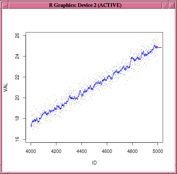
Description of "Figure 3-1 Fitted and Predicted Values Based on the esm.mod Model"
Example 3-38 builds a simple smoothing model based on a transactional data set. As preprocessing, it aggregates the values to the day level by taking averages, and fills missing values by setting them to the previous aggregated value. The model is then built on the aggregated daily time series. The function predict is invoked to generate predicted values on the daily basis.
Example 3-38 Building a Time Series Model with Transactional Data
ts01 <- data.frame(ID=seq(as.POSIXct("2008/6/13"), as.POSIXct("2011/6/16"),
                   length.out=4000), VAL=rnorm(4000, 10))
ts02 <- data.frame(ID=seq(as.POSIXct("2011/7/19"), as.POSIXct("2012/11/20"),
                   length.out=1500), VAL=rnorm(1500, 10))
ts03 <- data.frame(ID=seq(as.POSIXct("2012/12/09"), as.POSIXct("2013/9/25"),
                   length.out=1000), VAL=rnorm(1000, 10))
ts1 = ore.push(rbind(ts01, ts02, ts03))
rownames(ts1) <- ts1$ID
x <- ts1$VAL
esm.mod <- ore.esm(x, "DAY", accumulate = "AVG", model="simple",
                   setmissing="PREV")
esm.predict <- predict(esm.mod)
esm.predict
Listing for Example 3-38
R> ts01 <- data.frame(ID=seq(as.POSIXct("2008/6/13"), as.POSIXct("2011/6/16"),
+                      length.out=4000), VAL=rnorm(4000, 10))
R> ts02 <- data.frame(ID=seq(as.POSIXct("2011/7/19"), as.POSIXct("2012/11/20"),
+                     length.out=1500), VAL=rnorm(1500, 10))
R> ts03 <- data.frame(ID=seq(as.POSIXct("2012/12/09"), as.POSIXct("2013/9/25"),
+                     length.out=1000), VAL=rnorm(1000, 10))
R> ts1 = ore.push(rbind(ts01, ts02, ts03))
R> rownames(ts1) <- ts1$ID
R> x <- ts1$VAL
R> esm.mod <- ore.esm(x, "DAY", accumulate = "AVG", model="simple",
+                     setmissing="PREV")
R> esm.predict <- predict(esm.mod)
R> esm.predict
           ID      VAL
1  2013-09-26 9.962478
2  2013-09-27 9.962478
3  2013-09-28 9.962478
4  2013-09-29 9.962478
5  2013-09-30 9.962478
6  2013-10-01 9.962478
7  2013-10-02 9.962478
8  2013-10-03 9.962478
9  2013-10-04 9.962478
10 2013-10-05 9.962478
11 2013-10-06 9.962478
12 2013-10-07 9.962478
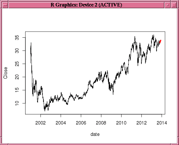
Figure 3-1 uses stock data from the TTR package. It builds a double exponential smoothing model based on the daily stock closing prices. The 30-day predicted stock prices, along with the original observations, are shown in Figure 3-2.
Example 3-39 Building a Double Exponential Smoothing Model Specifying an Interval
library(TTR)
stock <- "orcl"
xts.data <- getYahooData(stock, 20010101, 20131024)
df.data <- data.frame(xts.data)
df.data$date <- index(xts.data)
of.data <- ore.push(df.data[, c("date", "Close")])
rownames(of.data) <- of.data$date
esm.mod <- ore.esm(of.data$Close, "DAY", model = "double")
esm.predict <- predict(esm.mod, 30)
plot(of.data,type="l")
lines(esm.predict,col="red",lwd=4)
Ranking Data
The ore.rank function analyzes distribution of values in numeric columns of an ore.frame.
The ore.rank function supports useful functionality, including:
-
Ranking within groups
-
Partitioning rows into groups based on rank tiles
-
Calculation of cumulative percentages and percentiles
-
Treatment of ties
-
Calculation of normal scores from ranks
The ore.rank function syntax is simpler than the corresponding SQL queries.
The ore.rank function returns an ore.frame in all instances.
You can use these R scoring methods with ore.rank:
-
To compute exponential scores from ranks, use
savage. -
To compute normal scores, use one of
blom,tukey, orvw(van der Waerden).
For details about the function arguments, invoke help(ore.rank).
The following examples illustrate using ore.rank. The examples use the NARROW data set.
Example 3-40 ranks the two columns AGE and CLASS and reports the results as derived columns; values are ranked in the default order, which is ascending.
Example 3-41 ranks the two columns AGE and CLASS. If there is a tie, the smallest value is assigned to all tied values.
Example 3-41 Handling Ties in Ranking
x <- ore.rank(data=NARROW, var='AGE=RankOfAge, CLASS=RankOfClass', ties='low')
Example 3-42 ranks the two columns AGE and CLASS and then ranks the resulting values according to COUNTRY:
Example 3-42 Ranking by Groups
x <- ore.rank(data=NARROW, var='AGE=RankOfAge, CLASS=RankOfClass', group.by='COUNTRY')
Example 3-43 ranks the two columns AGE and CLASS and partitions the columns into deciles (10 partitions):
Example 3-43 Partitioning into Deciles
x <- ore.rank(data=NARROW, var='AGE=RankOfAge, CLASS=RankOfClass',groups=10)
To partition the columns into a different number of partitions, change the value of groups. For example, groups=4 partitions into quartiles.
Example 3-44 ranks the two columns AGE and CLASS and estimates the cumulative distribution function for both column.
Example 3-44 Estimating Cumulative Distribution Function
x <- ore.rank(data=NARROW, var='AGE=RankOfAge, CLASS=RankOfClass',nplus1=TRUE)
Example 3-45 ranks the two columns AGE and CLASS and scores the ranks in two different ways. The first command partitions the columns into percentiles (100 groups). The savage scoring method calculates exponential scores and blom scoring calculates normal scores:
Sorting Data
The ore.sort function enables flexible sorting of a data frame along one or more columns specified by the by argument.
The ore.sort function can be used with other data pre-processing functions. The results of sorting can provide input to R visualization.
The ore.sort function sorting takes places in the Oracle database. The ore.sort function supports the database nls.sort option.
The ore.sort function returns an ore.frame.
For details about the function arguments, invoke help(ore.sort).
Most of the following examples use the NARROW data set. There are also examples that use the ONTIME_S data set.
Example 3-46 sorts the columns AGE and GENDER in descending order.
Example 3-46 Sorting Columns in Descending Order
x <- ore.sort(data=NARROW, by='AGE,GENDER', reverse=TRUE)
Example 3-47 sorts AGE in descending order and GENDER in ascending order.
Example 3-47 Sorting Different Columns in Different Orders
x <- ore.sort(data=NARROW, by='-AGE,GENDER')
Example 3-48 sorts by AGE and keep one row per unique value of AGE:
Example 3-48 Sorting and Returning One Row per Unique Value
x <- ore.sort(data=NARROW, by='AGE', unique.key=TRUE)
Example 3-49 sorts by AGE and remove duplicate rows:
Example 3-50 sorts by AGE, removes duplicate rows, and returns one row per unique value of AGE.
Example 3-50 Removing Duplicate Columns and Returning One Row per Unique Value
x <- ore.sort(data=NARROW, by='AGE', unique.data=TRUE, unique.key = TRUE)
Example 3-51 maintains the relative order in the sorted output.
Example 3-51 Preserving Relative Order in the Output
x <- ore.sort(data=NARROW, by='AGE', stable=TRUE)
The following examples use the ONTIME_S airline data set. Example 3-52 sorts ONTIME_S by airline name in descending order and departure delay in ascending order.
Example 3-52 Sorting Two Columns in Different Orders
sortedOnTime1 <- ore.sort(data=ONTIME_S, by='-UNIQUECARRIER,DEPDELAY')
Example 3-53 sorts ONTIME_S by airline name and departure delay and selects one of each combination (that is, returns a unique key).
Summarizing Data
The ore.summary function calculates descriptive statistics and supports extensive analysis of columns in an ore.frame, along with flexible row aggregations.
The ore.summary function supports these statistics:
-
Mean, minimum, maximum, mode, number of missing values, sum, weighted sum
-
Corrected and uncorrected sum of squares, range of values,
stddev,stderr,variance -
t-test for testing the hypothesis that the population mean is 0
-
Kurtosis, skew, Coefficient of Variation
-
Quantiles: p1, p5, p10, p25, p50, p75, p90, p95, p99, qrange
-
1-sided and 2-sided Confidence Limits for the mean:
clm,rclm,lclm -
Extreme value tagging
The ore.summary function provides a relatively simple syntax compared with SQL queries that produce the same results.
The ore.summary function returns an ore.frame in all cases except when the group.by argument is used. If the group.by argument is used, then ore.summary returns a list of ore.frame objects, one ore.frame per stratum.
For details about the function arguments, invoke help(ore.summary).
Example 3-54 calculates the mean, minimum, and maximum values for columns AGE and CLASS and rolls up (aggregates) the GENDER column.
Example 3-54 Calculating Default Statistics
ore.summary(NARROW, class='GENDER', var ='AGE,CLASS', order='freq')
Example 3-55 calculates the skew of AGE as column A and the probability of the Student's t distribution for CLASS as column B.
Example 3-55 Calculating Skew and Probability for t Test
ore.summary(NARROW, class='GENDER', var='AGE,CLASS', stats='skew(AGE)=A, probt(CLASS)=B')
Example 3-56 calculates the weighted sum for AGE aggregated by GENDER with YRS_RESIDENCE as weights; in other words, it calculates sum(var*weight).
Example 3-56 Calculating the Weighted Sum
ore.summary(NARROW, class='GENDER', var='AGE', stats='sum=X', weight='YRS_RESIDENCE')
Example 3-57 groups CLASS by GENDER and MARITAL_STATUS.
Example 3-57 Grouping by Two Columns
ore.summary(NARROW, class='GENDER, MARITAL_STATUS', var='CLASS', ways=1)
Example 3-58 groups CLASS in all possible ways by GENDER and MARITAL_STATUS.
Analyzing Distribution of Numeric Variables
The ore.univariate function provides distribution analysis of numeric variables in an ore.frame.
The ore.univariate function provides these statistics:
-
All statistics reported by the
summaryfunction -
Signed rank test, Student's t-test
-
Extreme values reporting
The ore.univariate function returns an ore.frame as output in all cases.
For details about the function arguments, invoke help(ore.univariate).
Example 3-59 calculates the default univariate statistics for AGE, YRS_RESIDENCE, and CLASS.
Example 3-59 Calculating the Default Univariate Statistics
ore.univariate(NARROW, var="AGE,YRS_RESIDENCE,CLASS")
Example 3-60 calculates location statistics for YRS_RESIDENCE.
Example 3-60 Calculating the Default Univariate Statistics
ore.univariate(NARROW, var="YRS_RESIDENCE", stats="location")
Example 3-61 calculates complete quantile statistics for AGE and YRS_RESIDENCE.
Using a Third-Party Package on the Client
In Oracle R Enterprise, if you want to use functions from an open source R package from The Comprehensive R Archive Network (CRAN) or other third-party R package, then you would generally do so in the context of embedded R execution. Using embedded R execution, you can take advantage of the likely greater amount of RAM on the database server.
However, if you want to use a third-party package function in your local R session on data from an Oracle database table, you must use the ore.pull function to get the data from an ore.frame object to your local session as a data.frame object. This is the same as using open source R except that you can extract the data from the database without needing the help of a DBA.
When pulling data from a database table to a local data.frame, you are limited to using the amount of data that can fit into the memory of your local machine. On your local machine, you do not have the benefits provided by embedded R execution.
To use a third-party package, you must install it on your system and load it in your R session. Example 3-62 demonstrates downloading, installing, and loading the CRAN package kernlab. The kernlab package contains kernel-based machine learning methods. The example invokes the install.packages function to download and install the package. It then invokes the library function to load the package.
Example 3-62 Downloading, Installing, and Loading a Third-Party Package on the Client
install.packages("kernlab")
library("kernlab")
Listing for Example 3-62
R> install.packages("kernlab")
trying URL 'http://cran.rstudio.com/bin/windows/contrib/3.0/kernlab_0.9-19.zip'
Content type 'application/zip' length 2029405 bytes (1.9 Mb)
opened URL
downloaded 1.9 Mb

package 'kernlab' successfully unpacked and MD5 sums checked

The downloaded binary packages are in
        C:\Users\rquser\AppData\Local\Temp\RtmpSKVZql\downloaded_packages
R> library("kernlab")
Example 3-63 invokes the demo function to look for example programs in the kernlab package. Because the package does not have examples, Example 3-63 then gets help for the ksvm function. The example invokes example code from the help.
Example 3-63 Using a kernlab Package Function
demo(package = "kernlab")
help(package = "kernlab", ksvm)
data(spam)
index <- sample(1:dim(spam)[1])
spamtrain <- spam[index[1:floor(dim(spam)[1]/2)], ]
spamtest <- spam[index[((ceiling(dim(spam)[1]/2)) + 1):dim(spam)[1]], ]
filter <- ksvm(type~.,data=spamtrain,kernel="rbfdot",
+              kpar=list(sigma=0.05),C=5,cross=3)
filter
table(mailtype,spamtest[,58])
Listing for Example 3-63
> demo(package = "kernlab")
no demos found
> help(package = "kernlab", ksvm)    # Output not shown.
> data(spam)
> index <- sample(1:dim(spam)[1])
> spamtrain <- spam[index[1:floor(dim(spam)[1]/2)], ]
> spamtest <- spam[index[((ceiling(dim(spam)[1]/2)) + 1):dim(spam)[1]], ]
> filter <- ksvm(type~.,data=spamtrain,kernel="rbfdot",
+                kpar=list(sigma=0.05),C=5,cross=3)
> filter
Support Vector Machine object of class "ksvm"

SV type: C-svc  (classification)
 parameter : cost C = 5

Gaussian Radial Basis kernel function.
 Hyperparameter : sigma =  0.05

Number of Support Vectors : 970

Objective Function Value : -1058.218
Training error : 0.018261
Cross validation error : 0.08696
> mailtype <- predict(filter,spamtest[,-58])
> table(mailtype,spamtest[,58])

mailtype  nonspam spam
  nonspam    1347  136
  spam         45  772
For an example that uses the kernlab package, see Example 2-13, "Ordering Using Keys".