3.2.6 Building Exponential Smoothing Models on Time Series Data
The ore.esm function builds a simple or a double exponential smoothing model for in-database time series observations in an ordered ore.vector object. The function operates on time series data, whose observations are evenly spaced by a fixed interval, or transactional data, whose observations are not equally spaced. The function can aggregate the transactional data by a specified time interval, as well as handle missing values using a specified method, before entering the modeling phase.
The ore.esm function processes the data in one or more R engines running on the database server. The function returns an object of class ore.esm.
You can use the predict method to predict the time series of the exponential smoothing model built by ore.esm. If you have loaded the forecast package, then you can use the forecast method on the ore.esm object. You can use the fitted method to generate the fitted values of the training time series data set.
For information about the arguments of the ore.esm function, invoke help(ore.esm).
Example 3-37 Building a Double Exponential Smoothing Model
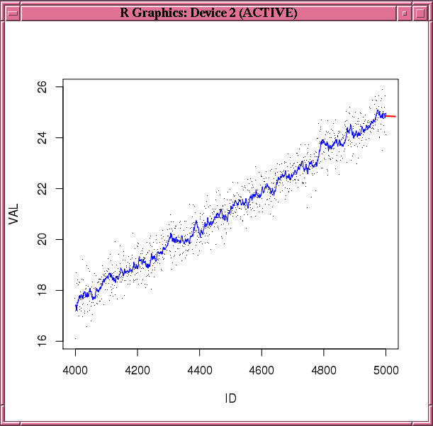
This example builds a double exponential smoothing model on a synthetic time series data set. The predict and fitted functions are invoked to generate the predictions and the fitted values, respectively. Figure 3-1 shows the observations, fitted values, and the predictions.
N <- 5000
ts0 <- ore.push(data.frame(ID=1:N,
                           VAL=seq(1,5,length.out=N)^2+rnorm(N,sd=0.5)))
rownames(ts0) <- ts0$ID
x <- ts0$VAL
esm.mod <- ore.esm(x, model = "double")
esm.predict <- predict(esm.mod, 30)
esm.fitted <- fitted(esm.mod, start=4000, end=5000)
plot(ts0[4000:5000,], pch='.')
lines(ts0[4000:5000, 1], esm.fitted, col="blue")
lines(esm.predict, col="red", lwd=2)
Figure 3-1 Fitted and Predicted Values Based on the esm.mod Model

Description of "Figure 3-1 Fitted and Predicted Values Based on the esm.mod Model"
Example 3-38 Building a Time Series Model with Transactional Data
This example builds a simple smoothing model based on a transactional data set. As preprocessing, it aggregates the values to the day level by taking averages, and fills missing values by setting them to the previous aggregated value. The model is then built on the aggregated daily time series. The function predict is invoked to generate predicted values on the daily basis.
ts01 <- data.frame(ID=seq(as.POSIXct("2008/6/13"), as.POSIXct("2011/6/16"),
                   length.out=4000), VAL=rnorm(4000, 10))
ts02 <- data.frame(ID=seq(as.POSIXct("2011/7/19"), as.POSIXct("2012/11/20"),
                   length.out=1500), VAL=rnorm(1500, 10))
ts03 <- data.frame(ID=seq(as.POSIXct("2012/12/09"), as.POSIXct("2013/9/25"),
                   length.out=1000), VAL=rnorm(1000, 10))
ts1 = ore.push(rbind(ts01, ts02, ts03))
rownames(ts1) <- ts1$ID
x <- ts1$VAL
esm.mod <- ore.esm(x, "DAY", accumulate = "AVG", model="simple",
                   setmissing="PREV")
esm.predict <- predict(esm.mod)
esm.predict
Listing for Example 3-38
R> ts01 <- data.frame(ID=seq(as.POSIXct("2008/6/13"), as.POSIXct("2011/6/16"),
+                      length.out=4000), VAL=rnorm(4000, 10))
R> ts02 <- data.frame(ID=seq(as.POSIXct("2011/7/19"), as.POSIXct("2012/11/20"),
+                     length.out=1500), VAL=rnorm(1500, 10))
R> ts03 <- data.frame(ID=seq(as.POSIXct("2012/12/09"), as.POSIXct("2013/9/25"),
+                     length.out=1000), VAL=rnorm(1000, 10))
R> ts1 = ore.push(rbind(ts01, ts02, ts03))
R> rownames(ts1) <- ts1$ID
R> x <- ts1$VAL
R> esm.mod <- ore.esm(x, "DAY", accumulate = "AVG", model="simple",
+                     setmissing="PREV")
R> esm.predict <- predict(esm.mod)
R> esm.predict
           ID      VAL
1  2013-09-26 9.962478
2  2013-09-27 9.962478
3  2013-09-28 9.962478
4  2013-09-29 9.962478
5  2013-09-30 9.962478
6  2013-10-01 9.962478
7  2013-10-02 9.962478
8  2013-10-03 9.962478
9  2013-10-04 9.962478
10 2013-10-05 9.962478
11 2013-10-06 9.962478
12 2013-10-07 9.962478
Example 3-39 Building a Double Exponential Smoothing Model Specifying an Interval
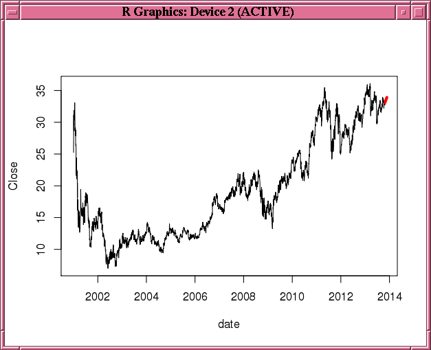
This example uses stock data from the TTR package. It builds a double exponential smoothing model based on the daily stock closing prices. The 30-day predicted stock prices, along with the original observations, are shown in Figure 3-2.
library(TTR)
stock <- "orcl"
xts.data <- getYahooData(stock, 20010101, 20131024)
df.data <- data.frame(xts.data)
df.data$date <- index(xts.data)
of.data <- ore.push(df.data[, c("date", "Close")])
rownames(of.data) <- of.data$date
esm.mod <- ore.esm(of.data$Close, "DAY", model = "double")
esm.predict <- predict(esm.mod, 30)
plot(of.data,type="l")
lines(esm.predict,col="red",lwd=4)
