| Oracle® Retail Demand Forecasting Cloud Service User Guide Release 19.0 F24922-17 |
|

 Previous |
 Next |
| Oracle® Retail Demand Forecasting Cloud Service User Guide Release 19.0 F24922-17 |
|
Previous |
Next |
This chapter describes the Estimation Setup Short Lifecycle for RDF Cloud Service.
The following table lists the workspaces, steps, and views for the Estimation Setup Short Lifecycle task.
The General Estimation Setup SLC workspace allows you access to all of the views listed in Estimation Setup SLC Workspaces, Steps, and Views.
To build the General Estimation Setup SLC workspace, perform these steps:
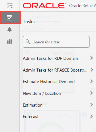
From the left sidebar menu, click the Task Module to view the available tasks.
Click the Estimation activity and then click Setup to access the available workspaces.
Click Short Lifecycle. The Short Lifecycle wizard opens.
You can open an existing workspace, but to create a new workspace, click Create New Workspace.
Enter a name for your new workspace in the label text box and click OK.
The Workspace wizard opens. Select the products you want to work with and click Next.
Select the locations you want to work with and click Finish.
The wizard notifies you that your workspace is being prepared. Successful workspaces are available from the Dashboard.
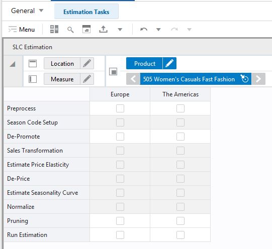
This step includes the SLC Estimation Setup View.
The SLC Estimation Setup view shows the steps running the estimation and allows enabling or disabling some of them.
The SLC Estimation view contains the following measures:
Run Estimation
If this flag is selected, estimation is run for the given merchandise.
Preprocess
If this flag is selected, preprocessing is run for the given merchandise. During this step unreliable data points are filtered out and not considered in further calculations.
De-Price
During this step clearance effects are removed from the demand. De-pricing is mandatory.
De-Promote
If this flag is selected the demand is depromoted. During this step, the effects of temporary price reductions of promotions and holidays are removed from demand.
Normalize
During this step the lifecycle curves are normalized, so the values add up to 52. Normalizing is mandatory.
Estimate Price Elasticity
During this step the impact of clearance prices on demand are quantified. The outputs are price elasticities. Estimating price elasticities is mandatory
Season Code Setup
During this step the user defines how merchandise shall be grouped so its demand is processed together. Setting up season codes is mandatory.
Estimate Seasonality Curve
During this step seasonality curves are calculated at several escalation levels. Estimating seasonality curves is mandatory.
Sales Transformation
During this step the sales are processed such that seasonality and other effects are removed. Sales transformation is mandatory.
History End Date
In this measure the user can specify the most recent period to be used in estimation. For instance if today's date is 1/1/2025, and the user sets the History End Date to be 12/1/2024, the sales from December 2024 are not used during estimation.
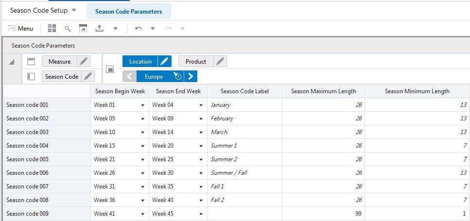
This step includes the Season Code Parameters View.
The goal of the estimation task is to estimate seasonality curves as well as price and promotion effects. Since short lifecycle merchandise, such as fashion items, do not sell year over year, demand for the items that are selling this year, is not available for past years. The demand parameters need to be estimated using demand of similar items that sold in previous years.
Among the criteria used for deciding what similar items are, include the following:
When the items have started selling
How long the items have been selling
For instance, a possible scenario is to group all items that have started selling in March, and have been selling for 13 weeks. Or all items that have started selling in Spring and sold for up to 26 weeks. All items that share these properties are sharing a so called season code
In the Season Code Parameters view, you can specify the basic information for defining season codes.
|
Note: An item/location can only belong to one season code. |
The Season Code Parameters view contains the following measures:
Season Begin Week
The Season Begin Week and Season End Week define the period that similar items start selling. For instance, we may say that items starting selling in the second half of March and beginning of April should be considered to belong to the same season code. Note that in addition to the period when items start selling, the season length criteria also needs to be met.
Season End Week
The Season Begin Week and Season End Week define the period that similar items start selling. For instance, we may say that items starting selling in the second half of March and beginning of April should be considered to belong to the same season code. Note that in addition to the period when items start selling, the season length criteria also needs to be met.
Season Code Label
This measure allows you to give a meaningful label to items that are processed together. For instance 'Spring Fast Fashion' or 'Winter Apparel'.
Season Maximum Length
The Season Minimum and Maximum Length measures allow the grouping of items by the length of their shelf life. For instance items that sell between 10 and 15 weeks are candidates to be grouped together in the same season code. Note that for the grouping to actually happen the items also need to start selling around the same time of the year, as defined by the Season Begin and End measures.
Season Minimum Length
The Season Minimum and Maximum Length measures allow the grouping of items by the length of their shelf life. For instance items that sell between 10 and 15 weeks are candidates to be grouped together in the same season code. Note that for the grouping to actually happen the items also need to start selling around the same time of the year, as defined by the Season Begin and End measures.
The available views are:
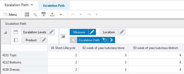
The Default Escalation Path view allows you to specify the priority of each escalation level. Escalation levels with low intersections, such as subclass, usually capture more detailed demand patterns, but are less stable because the lower number of data points used for estimation.
Escalation levels with high intersections, such as department, usually capture more generic demand patterns, but are very stable because of the large number of data points used for estimation.
The Default Escalation Path view contains the following measures:
Level Intersection
This measure displays the intersections of the escalation levels. This can be helpful for the business user when assigning priorities in the escalation path.
Escalation Path
The user can specify the priority in which the system searches escalation levels for forecast parameters like seasonality curves and/or promotion effects. For instance, suppose there are three escalation levels available. The path may be defined as follows:
Escalation Level #1: priority 3
Escalation Level #2: priority 4
Escalation Level #3: priority 2
In this case, when generating the forecast, the system will first look to get parameters from Escalation Level #3 (highest priority). If they are available, they are used. If they are not available, because they were deemed unreliable and pruned, the system will go to Escalation Level #1 (second highest priority). Finally, if the search is not successful, the search continues at Escalation Level #2.
This step includes the Estimation Parameters Sub-step.
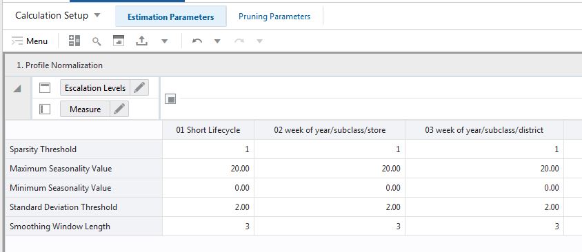
This sub-step includes the Profile Normalization View.
The Profile Normalization view explains the filters or checks that a curve needs to pass.
The Profile Normalization view contains the following measures:
Sparsity Threshold
Seasonality curves with the number of consecutive periods with indices equal to zero equal to or less than the sparsity threshold will be pruned.
Maximum Seasonality Value
This number holds the maximum allowed seasonality value.
Minimum Seasonality Value
This number holds the minimum allowed seasonality value.
Standard Deviation Threshold
This measure holds the maximum allowed standard deviation of the curve.
Smoothing Window Length
Window length for smoothing using the Standard Median filter.
The Filter Thresholds view explains the pruning strategy.
After estimation is performed, the demand parameters are undergoing a rigorous check to make sure they are suitable for forecasting. In this view, you can set the thresholds for various filters.
The Filter Thresholds view contains the following measures:
Season Ratio Threshold
This measure defines the length of the season. If the sales are less than the maximum sales times this threshold, the sales are not used in further calculations.
Max Number of Zero Sales
This is maximum allowed number of zero sales cells that a curve can have without being pruned.
Average Sales Threshold
This is the minimum allowed average sales that a curve can have without being pruned.
Minimum Weeks Threshold
This is the minimum allowed number of weeks that a curve must have data for without being pruned.
Season Length Threshold
This measure decides which sales to use in further calculations. If the season length for a product location combination is less than this value, the sales of the product location combination are not used in further calculations.
Season Length Upper Bound
This measure controls the upper bound of the sales length to be used in the Short Lifecycle calculation. Items with sales count greater than the season length upper bound will be pruned out.
The pruned time series based on the Season Length threshold and season length upped bound will be displayed in the SLC Preprocess Summary in the Estimation Review workbook.
Markdown Upper Bound
This measure decides if a marked down period is a legitimate data point or must be discarded. If the sales price for the period divided by the regular price is more than this value, the data point is discarded.
Markdown Lower Bound
This measure decides if a marked down period is a legitimate data point or must be discarded. If the sales price for the period divided by the regular price is less than this value, the data point is discarded.
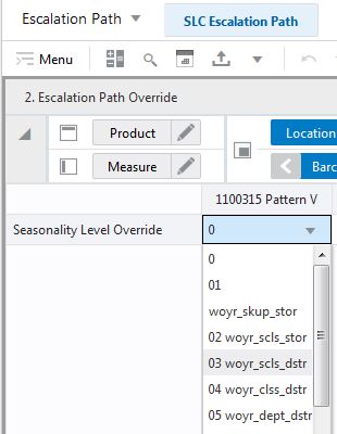
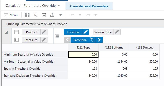
This step includes the Pruning Parameters Override View.
In the Pruning Parameters Override view you can override the thresholds for the pruning thresholds at a more granular level.
The Pruning Parameters Override view contains the following measures:
Minimum Seasonality Value Override
This number holds the minimum allowed seasonality value. If set to zero, it assures that no negative seasonal indices are used.
Maximum Seasonality Value Override
This number holds the maximum allowed seasonality value.
Sparsity Threshold Override
Override of the Sparsity Threshold value.
Standard Deviation Threshold Override
This measure holds the maximum allowed standard deviation of the curve.
The available views are:
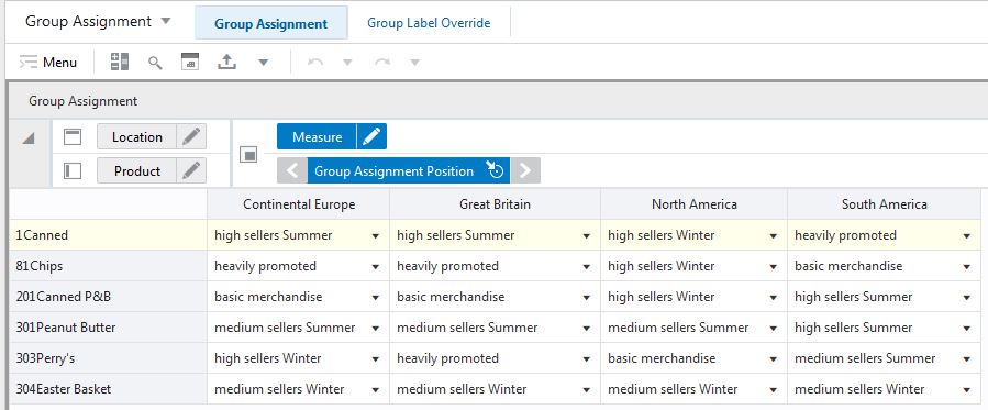
Typically, escalation and pooling levels are intersections along the product, location and calendar hierarchies, such as subclass/region/week. However, RDFCS also offers the ultimate flexibility where any item at any store can be grouped together. For instance rain gear in the Southeast region, may be grouped together with snow shovels in the Midwest region, something that would not be possible if the levels are tied to the hierarchies. Determining what item/locations is meaningful to be grouped together can be achieved in several ways. First, the analysis can be done outside of RDFCS, and the groups can be imported using Load Measure. A second option is to implement logic in RDFCS thru the extensibility framework. Finally, the Group Assignment view allows you to manually assign time series to such groups.
The Group Assignment view contains the following measures:
Group Assignment
Use these measures to specify the group that certain product/location combinations belong to. Note that multiple Group Assignment measures are available. Consider a red shirt selling at a large store at the outskirts of a large metro area. This item/store combination can be part of a certain group where the clustering is done by merchandise. It could potentially be grouped together with other basic fashion items. A different clustering can be done by price tier and store format. There it could be grouped together with other medium priced items selling at a large store.
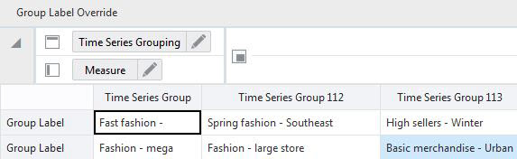
Typically, the groups and their labels are handled outside the solution. However, if no proper labels were specified, they can be overwritten in this view.
The Group Label Override view contains the following measures:
Group Label
These measures allow you to specify labels that describe grouping criteria of item and locations combinations that are assigned to it. There are as many Group Label measures as there are Group Assignment measures.