| Oracle® Retail Demand Forecasting Cloud Service User Guide Release 19.0 F24922-17 |
|

 Previous |
 Next |
| Oracle® Retail Demand Forecasting Cloud Service User Guide Release 19.0 F24922-17 |
|
Previous |
Next |
This chapter describes the Estimation Setup Long Lifecycle for RDF Cloud Service.
The following table lists the workspaces, steps, and views for the Estimation Setup Long Lifecycle task.
The General Estimation Setup LLC workspace allows you access to all of the views listed in Estimation Setup LLC Workspaces, Steps, and Views.
To build the General Estimation Setup LLC workspace, perform these steps:
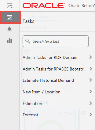
From the left sidebar menu, click the Task Module to view the available tasks.
Click the Estimation activity and then click Setup to access the available workspaces.
Click Long Lifecycle. The Long Lifecycle wizard opens.
You can open an existing workspace, but to create a new workspace, click Create New Workspace.
Enter a name for your new workspace in the label text box and click OK.
The Workspace wizard opens. Select the products you want to work with and click Next.
Select the locations you want to work with and click Finish.
The wizard notifies you that your workspace is being prepared. Successful workspaces are available from the Dashboard.
In this step, you can adjust parameters that determine the strategy around how to create seasonality curves. For example. you can decide which estimation method to use and tweak certain parameters that are relevant to the estimation method.
This step includes these sub-steps:
The measures in the Global Parameters view are level or intersection specific. For example, for a certain intersection; the estimation method can be Auto_Seasonal, while for other levels it can be set to Blend_Seasonal.
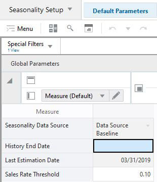
The Global Parameters view contains the following measures:
Seasonality Data Source
This measure displays the name of the data source used to create seasonality curves.
History End Date
In this measure the user can specify the most recent period to be used in estimation. For instance if today's date is 1/1/2025, and the user sets the History End Date to be 12/1/2024, the sales from December 2024 are not used during estimation.
Last Estimation Date
This measure displays the last time estimation was run. The date can be an indication if the forecast parameters should be refreshed by rerunning estimation.
Sales Rate Threshold
In this measure you can specify the sales rate that determines if the demand should be de-seasonalized or if the step should be skipped.
For items selling on average more than the threshold value, the demand is de-seasonalized before the base rate of demand is calculated. However, for slow selling items, de-seasonalizing the demand can lead to inflated forecast. Hence, if an item is selling less than the value listed in this measure, the base rate of demand is calculated based on the demand, skipping the de-seasonalizing step.
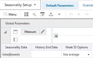
The measures in the Level Parameters view are at a very high intersection and can be overwritten at a more granular level.
The Level Parameters view contains the following measures:
History Start Date
This field indicates to the system the point in the historical sales data at which to use in the forecast generation process. If no date is indicated, the system defaults to the first date in your calendar. It is also important to note that the system ignores leading zeros that begin at the history start date. For example, if your history start date is January 1, 2017 and an item/location does not have sales history until February 1, 2017, the system considers the starting point in that item/location's history to be the first data point where there is a non-zero sales value.
Estimate Method
Use this measure to specify the method used in the seasonality estimation. The choices are:
ORACLE_AWINTERS
REGULAR_AWINTERS
ORACLE_MWINTERS
REGULAR_AWINTERS
AUTO_SEASONAL
BLEND_SEASONAL
Winters Max Alpha
In the Winters (SeasonalES) model-fitting procedure, alpha (a model parameter capturing the level) is determined by optimizing the fit over the time series. This field displays the maximum value (cap value) of alpha allowed in the model-fitting process. An alpha cap value closer to one (1) allows more reactive models (alpha = 1, repeats the last data point), whereas alpha cap closer to zero (0) only allows less reactive models. The default is one (1).
Minimum Winters Data Points
The value in this field is the minimum number of periods of historical data necessary for Winters to be considered as a potential forecast method. If not enough years of data are available for a given time series, Winters is not used. The system default is two years of required history, which corresponds two full sales cycles. The value must be set based on the calendar dimension of the level. For example, if the calendar dimension is week, the value is 104.
Seasonal Smooth Index
This parameter is used in the calculation of seasonal index. The current default value used within forecasting is 0.80. Changes to this parameter impacts the value of seasonal index directly and impact the level indirectly. When seasonal smooth index is set to one (1), seasonal index is closer to the seasonal index of last year sales. When seasonal smooth index is set to zero (0), seasonal index is set to the initial seasonal indexes calculated from history.
Winters Max Gamma
In the Winters (SeasonalES) model-fitting procedure, gamma (a model parameter capturing the trend) is determined by optimizing the fit over the time series. This field displays the maximum value (cap value) of gamma allowed in the model-fitting process.
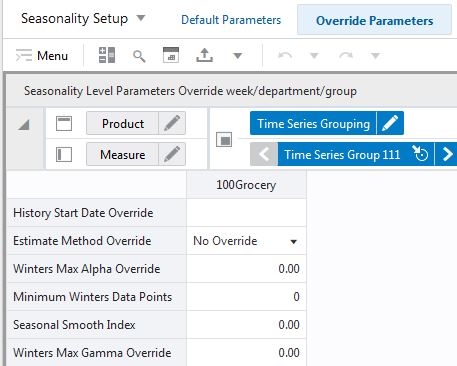
The Seasonality Level Parameters Override view allows you to override the parameters at each position of any level. For instance, if the level is department, the for one department the estimation method may be AUTO_SEASONAL, and for others it may be BLEND_SEASONAL.
The Seasonality Level Parameters Override view contains the following measures:
History Start Date Override
This parameter represents the first point in time from which the Forecasting Engine begins training and modeling (that is, if there are two years of history, but you only want to use one year, you set the start date to a year ago). This parameter overrides the History Start Date to the desired item/location intersection. For example, if you have a large spike in the first three weeks of sales for an item on sale, you can set the Historical Start Date to one week past that period, and those first few weeks are not used when generating the forecast.
It is also important to note that the system ignores leading zeros that begin at the history start date. For example, if your history start date is January 1, 2003, and an item/location does not have sales history until February 1, 2003, the system considers the starting point in that item/location's history to be the first data point where there is a non-zero sales value.
If this parameter is set into the future, there would be no forecast, as the history training window is read as zero.
Estimate Method Override
Use this measure to override the method used in the seasonality estimation. The choices are:
ORACLE_AWINTERS
REGULAR_AWINTERS
ORACLE_MWINTERS
REGULAR_AWINTERS
AUTO_SEASONAL
BLEND_SEASONAL
Winters Max Alpha Override
This is the override of the default Winters Max Alpha value.
Minimum Winters Data Points Override
This is the override of the default Minimum Winters Data Points value.
Seasonal Smooth Index Override
This is the override of the Seasonal Smooth Index value.
Winters Max Gamma Override
This is the override of the Winters Max Gamma value.
This step includes these sub-steps:
The Global Parameters view allows you to specify the strategy for estimating promotion and price effects. The strategy can be defined at a high, or global level, and can be overwritten at more granular levels
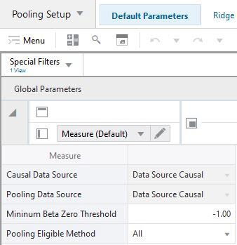
The Global Parameters view contains the following measures:
Causal Data Source
This measure displays the name of the data source used to calculate promotion effects at the final level.
Pooling Data Source
This measure displays the name of the data source used to calculate promotion effects at the pooling levels. The measure may be different than the causal data source, because at the pooling levels the data source can be normalized, something that is not recommended for the final level.
Minimum Beta Zero Threshold
This parameter specifies the minimum value of the intercept calculated during regression. If a number is less that the threshold, the estimates are considered unstable.
Pooling Eligible Method
This measure allows you to control which time series are used to estimate promotion effects at pooling levels.
The available options are
All: all time series are used to estimate promotion effects at pooling levels. Note that time series that were not promoted in history are automatically excluded from the estimation.
Relevant Only: only time series that have relevant promotion effects at the final level are used in the estimation at pooling levels. These time series have final effects determined by the blending of pooling and final level effects. Time series without relevant effects at the final level will use pooling effects.
Custom: The third option is to write custom rules to determine which time series should contribute to the pooling levels estimation.
For instance, you can specify that all low sellers are excluded from the estimation. Or you can reject all time series that are promoted more that 90% of the time. Or time series that sell only when they are promoted..
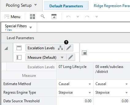
The Level Parameters view allows you to specify the promotion and price estimation strategy at the pooling level.
The Level Parameters view contains the following measures:
Estimate Method
This measure allows you to specify if parameters should be estimated or not. The choices are
Causal: in which case parameters will be estimated
No Estimate: no promotion-related parameters will be estimated
A common reason why a user may not want to estimate promotion effects for certain item/locations is because the effects are still up to date, and do not need to be refreshed.
Regress Engine Type
This measure allows you to specify the mode of the regression engine. The options are:
Stepwise: Step-wise regression is used to estimate promotion and price effects
Ridge: Ridge regression is used to estimate promotion and price effects.
The Step-wise regression is a good candidate when promotions and price change instances are infrequent, such as at the item/store level. The step-wise first discards the events that it finds insignificant, and estimates effects for the significant ones.
The Ridge regression is a good candidate for the pooling levels where instances of events and price changes are plenty. The method is emphasizing stable events and punishing less significant.
Data Source Threshold
This measure allows you to specify the minimum value of the data source that is used in the calculations. It is recommended that the value is at least 1, so the estimation of events and price effect is robust and correctly reflects the impact on demand.
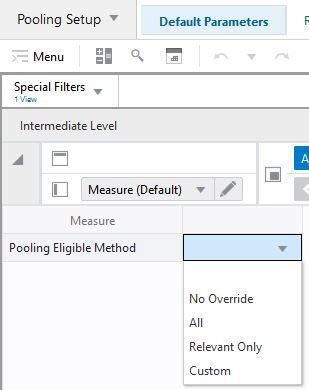
This view allows you to determine the pooling eligibility method at an intersection that is lower than global.
The Pooling Intermediate Parameters view contains the following measure:
Pooling Eligible Method
This measure allows you to control which time series are used to estimate promotion effects at pooling levels.
The available options are
All: all time series are used to estimate promotion effects at pooling levels. Note that time series that were not promoted in history are automatically excluded from the estimation.
Relevant Only: only time series that have relevant promotion effects at the final level are used in the estimation at pooling levels. These time series have final effects determined by the blending of pooling and final level effects. Time series without relevant effects at the final level will use pooling effects.
Custom: The third option is to write custom rules to determine which time series should contribute to the pooling levels estimation.
For instance, you can specify that all low sellers are excluded from the estimation. Or you can reject all time series that are promoted more that 90% of the time. Or time series that sell only when they are promoted.
The Promotion Model Type view allows you to enable or disable promotions effect estimation and determine the type of promotions.
The Promotion Model Type View view contains the following measures:
Promotion Effects Type
This measure allows you to view and select the type of promotion effects. If a promotion, for instance, front cap, is defined as real, the type is displayed as linear. If another event is defined as real, such as price discount, you can decide to estimate it using an exponential model or using the power law.
Enabled Promotion
This measure indicates if an event is enabled or not. If it is enabled, the system will attempt to quantify its effect on demand during the estimation task
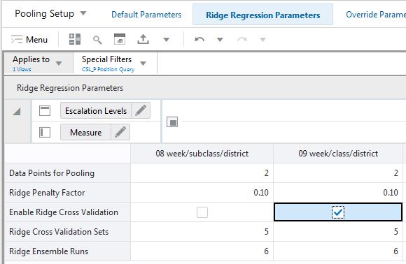
The Ridge Regression Parameters view allows you to select settings relevant to ridge regression.
The Ridge Regression Parameters view contains the following measures:
Data Points for Pooling
Ridge Penalty Factor
Enable Ridge regression Cross Validation
Ridge Regression Validation Sets
Ridge Ensemble Runs
These measures are fully detailed in the My Oracle Support white paper, Effects Estimation.
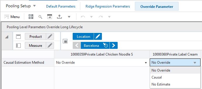
The Pooling Level Parameters Override view allows you to override the promotion effect estimation strategy at more granular levels.
The Pooling Level Parameters Override view contains the following measures:
Causal Estimation Method Override
This measure allows you to override the causal estimation method. The options are:
No override: default setting applies
Causal: effect estimation is performed
No estimate: effect estimation is not performed
This step includes these sub-steps:
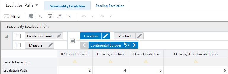
The Seasonality Escalation Path view allows you to specify the priority of each escalation level. Escalation levels with low intersections, such as subclass, usually capture more detailed seasonality patterns, but are less stable because the lower number of data points used for estimation.
Escalation levels with high intersections, such as department, usually capture more generic seasonality patterns, but are very stable because of the large number of data points used for estimation.
The Seasonality Escalation Path view contains the following measures:
Level Intersection
This measure displays the intersections of the escalation levels. This can be helpful for the business user when assigning priorities in the escalation path.
Escalation Path
The user can specify the priority in which the system searches escalation levels for seasonality curves. For instance, suppose there are three escalation levels available. The path may be defined as follows:
Escalation Level #1: priority 3
Escalation Level #2: priority 4
Escalation Level #3: priority 2
In this case, when generating the forecast, the system will first look to get parameters from Escalation Level #3 (highest priority). If the are available, they are used. If they are not available, because they were deemed unreliable and pruned, the system will go to Escalation Level #1 (second highest priority). Finally, if the search is not successful, the search continues at Escalation Level #2.
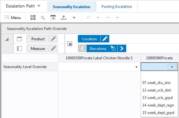
The Seasonality Escalation Path Override view allows you to override the escalation path for seasonality estimation.
The Seasonality Escalation Path Override view contains the following measures:
Escalation Path Override
In this field the user can override the default escalation path selections. She can enter the preferred Escalation Level, and that will become the top priority. However, if the forecast parameters for that level were deemed unreliable and pruned, the search will follow the default escalation path.
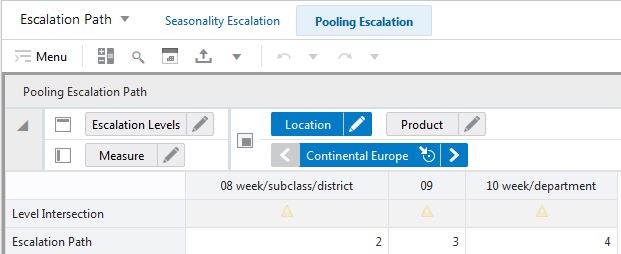
The Pooling Escalation Path view allows you to specify the priority of each escalation level. Escalation levels with low intersections, such as subclass, usually capture more detailed pooled effects, but are less stable because the lower number of data points used for estimation.
Escalation levels with high intersections, such as department, usually capture more generic pooling effects, but are very stable because of the large number of data points used for estimation.
The Pooling Escalation Path view contains the following measures:
Level Intersection
This measure displays the intersections of the pooling levels. This can be helpful for the business user when assigning priorities in the escalation path.
Escalation Path
The user can specify the priority in which the system searches pooling levels for promotion effects. For instance, suppose there are three escalation levels available. The path may be defined as follows:
Pooling Level #1: priority 3
Pooling Level #2: priority 4
Pooling Level #3: priority 2
In this case, when generating the forecast, the system will first look to get parameters from Escalation Level #3 (highest priority). If the are available, they are used. If they are not available, because they were deemed unreliable and pruned, the system will go to Escalation Level #1 (second highest priority). Finally, if the search is not successful, the search continues at Escalation Level #2.
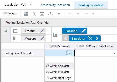
The Pooling Escalation Path Override view allows you to override the escalation path for pooling estimation.
The Pooling Escalation Path Override view contains the following measures:
Escalation Path Override
In this field the user can override the default escalation path selections. She can enter the preferred Pooling Level, and that will become the top priority. However, if the forecast parameters for that level were deemed unreliable and pruned, the search will follow the default escalation path.
This step includes these sub-steps:
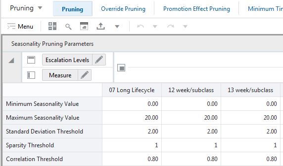
After seasonality estimation is performed, the seasonality curves are undergoing a rigorous check to make sure they are suitable for forecasting. Using the Seasonality Pruning Parameters view, you can set the thresholds for various filters.
The Seasonality Pruning Parameters view contains the following measures:
Minimum Seasonality Value
This number holds the minimum allowed seasonality value.
Maximum Seasonality Value
This number holds the maximum allowed seasonality value.
Standard Deviation Threshold
This measure holds the maximum allowed standard deviation of the curve.
Sparsity Threshold
Seasonality curves with the number of consecutive periods with indices equal to zero equal to or less than the sparsity threshold will be pruned.
Correlation Threshold
This measure holds the minimum allowed value of the correlation between the seasonality curve and the data source.
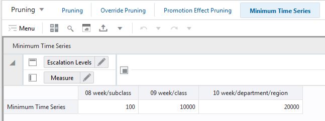
This step contains this view:
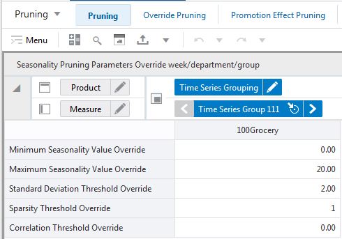
The Seasonality Pruning Parameters Override view allows you to override the threshold values for the pruning filters.
The Seasonality Pruning Parameters Override view contains the following measures:
Minimum Seasonality Value Override
Override of the Minimum Seasonality value.
Maximum Seasonality Value Override
Override of the Maximum Seasonality value.
Standard Deviation Threshold Override
Override of the Standard Deviation Threshold value.
Sparsity Threshold Override
Override of the Sparsity Threshold value.
Correlation Threshold Override
Override of the Correlation Threshold value.
After pooling estimation is performed, the promotion effects are undergoing a check to make sure they are suitable for forecasting. The Pooling Pruning Parameters allows you to set the thresholds for various filters.
The Pooling Pruning Parameters view contains the following measures:
Maximum Promo Effect
This measure holds the maximum allowed promo effect.
Minimum Promo Effect
This measure holds the minimum allowed promo effect.
Pruning Type
This measure specifies how pruning should work for the set of promotions at a given pooling level. The options are:
Single: If at a given pooling level, one particular effect does not pass the criteria of minimum or maximum allowed effects, it is pruned.
All: If at a given pooling level. one or more effects do not pass the criteria of minimum or maximum allowed effects, the effects of all promotions at that pooling level are pruned.
|
Note: Since this measure is set for all promotions at a pooling level, you need to roll up to all promotions to be able to edit the measure. |
The available views are:
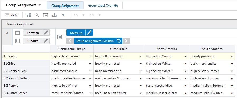
Typically, escalation and pooling levels are intersections along the product, location and calendar hierarchies, such as subclass/region/week. However, RDFCS also offers the ultimate flexibility where any item at any store can be grouped together. For instance rain gear in the Southeast region, may be grouped together with snow shovels in the Midwest region, something that would not be possible if the levels are tied to the hierarchies. Determining what item/locations is meaningful to be grouped together can be achieved in several ways. First, the analysis can be done outside of RDFCS, and the groups can be imported using Load Measure. A second option is to implement logic in RDFCS thru the extensibility framework. Finally, the Group Assignment view allows you to manually assign time series to such groups.
The Group Assignment view contains the following measures:
Group Assignment
Use these measures to specify the group that certain product/location combinations belong to. Note that multiple Group Assignment measures are available. Consider a red shirt selling at a large store at the outskirts of a large metro area. This item/store combination can be part of a certain group where the clustering is done by merchandise. It could potentially be grouped together with other basic fashion items. A different clustering can be done by price tier and store format. There it could be grouped together with other medium priced items selling at a large store.
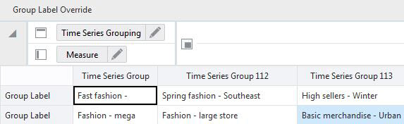
Typically, the groups and their labels are handled outside the solution. However, if no proper labels were specified, they can be overwritten in this view.
The Group Label Override view contains the following measures:
Group Label
These measures allow you to specify labels that describe grouping criteria of item and locations combinations that are assigned to it. There are as many Group Label measures as there are Group Assignment measures.