| Oracle® Retail Demand Forecasting Cloud Service User Guide Release 19.0 F24922-17 |
|

 Previous |
 Next |
| Oracle® Retail Demand Forecasting Cloud Service User Guide Release 19.0 F24922-17 |
|
Previous |
Next |
This chapter describes the Forecast Setup Long Lifecycle task for RDF Cloud Service.
The following table lists the workspaces, steps, and views for the Forecast Setup Long Lifecycle task.
The Forecast Setup LLC workspace allows you access to all of the views listed in Forecast Setup LLC Workspace.
To build the Forecast Setup LLC workspace, perform these steps:
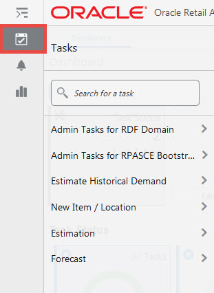
From the left sidebar menu, click the Task Module to view the available tasks.
Click the Forecast activity and then click Setup to access the available workspaces.
Click Long Lifecycle. The Long Lifecycle wizard opens.
You can open an existing workspace, but to create a new workspace, click Create New Workspace.
Enter a name for your new workspace in the label text box and click OK.
The Workspace wizard opens. Select the products you want to work with and click Next.
Select the locations you want to work with and click Finish.
The wizard notifies you that your workspace is being prepared. Successful workspaces are available from the Dashboard.
The Forecast Setup LLC workspace is built. This workspace contains these steps:
The available views are:
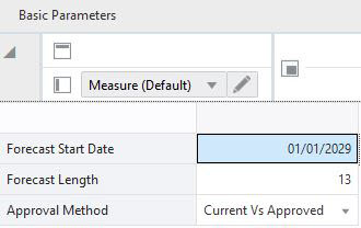
The Basic Parameters view allows you to view and set high level information. For instance, you can set the approval policy or determine the time frame for which forecast is required.
The Basic Parameters view contains the following measures:
Forecast Start Date
This is the starting date of the forecast. If no value is specified at the time of forecast generation, the system uses the data/time at which the batch is executed as the default value. If a value is specified in this field and it is used to successfully generate the batch forecast, this value is cleared.
Forecast Length
The Forecast Length is used with the Forecast Start Date to determine forecast horizon. The forecast length is based on the calendar dimension of the final-level. For example, if the forecast length is to be 10 weeks, the setting for a final-level at day is 70 (10 x 7 days).
Approval Method
This field is a list from which you select the default automatic approval policy for forecast items. Valid values are:
Manual
The system-generated forecast is not automatically approved. Forecast values must be manually approved by accessing and amending the Forecast Review view
Automatic
The system-generated quantity is automatically approved as is.
By Alert
This list of values may also include any Forecast Approval alerts that have been configured for use in the forecast approval process. Alerts are configured during the implementation and can be enabled to be used for Forecast Approval in the Enable Alert for Forecast Approval view. Refer to the Oracle Retail Predictive Application Server Configuration Tools User Guide for more information on the Alert Manager. The Alert Parameters view contains a list and descriptions of available alerts, and for which level (causal/baseline) that they are designed for.
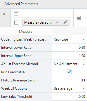
The Advanced Parameters view allows you to set default values for parameters that are less frequently accessed, such as History startdate or measures affecting cumulative interval calculations.
The Advanced Parameters view contains the following measures:
History Prerange Length
This measure lets you control how many calendar positions are showed in the wizard prior to RPAS_TODAY when building the Forecast Review workbook.
The historical positions (before RPAS_TODAY/forecast start date) displayed in the wizard are decided by the number entered here, and the history length used to forecast the level.
If the number displayed here is 10 and the history length is 17, the number of positions before today, are pre-ranged in the wizard to:
MAX (History Prerange Length, History Length) = MAX (10, 17) = 17
Adjust Forecast Method
This measure allows you to choose how to automatically adjust the system generated forecast. The options are:
No Adjustment
No adjustment is made to the system generated forecast
Keep Last Change
If any adjustments were done to the forecast in the previous runs, they are reflected in the Adjusted Forecast measure. In this use case, the total forecast is retained.
Keep Last Baseline
If any adjustments were done in the Adjusted Baseline in the previous runs, they are retained. In this use case. the system calculated peaks are applied on the Adjusted Baseline
Keep Last Peak
If any adjustments were done in the Adjusted Peak measure in the previous runs, they are retained. In this use case, the adjusted peaks are applied on the system calculated baseline.
Low Sales Threshold
In this measure you can specify the sales rate that determines if the demand should be de-seasonalized or if the step should be skipped.
Demand Transference
If Demand Transference is enabled in the plug-ins, and the necessary data is interfaced to RDFCS, and significant demand transference effects are detected, this options incorporates demand transference effects in the adjusted forecast. If demand transference effects are not zero, the system and adjusted forecasts will be different.
|
Note: The Demand Transference effects are calculated outside RDFCS. A good candidate is ORASE, the Oracle Retail science platform |
|
Note: Tables (UNKNOWN STEP NUMBER) , (UNKNOWN STEP NUMBER) , and (UNKNOWN STEP NUMBER) provide details for measure calculations for options selected in Forecast Setup. |
Updating Last Week Forecast
This field is a list from which you can select the method for updating the Approved Forecast for the last specified number of weeks of the forecast horizon. This option is valid only if the Approval Method Override is set to Manual or Approve by alert, and the alert was rejected. The choices are:
No change
When using this method, the last week in the forecast horizon does not have an Approved Forecast value. The number of weeks is determined number of weeks elapsed between the forecast start date and the last approval date.
Replicate
When using this method the last weeks in the forecast horizon are forecast using the Approved Forecast for the week corresponding to the last approval date.
Use Forecast
When using this method, the System Forecast for the last weeks in the forecast horizon is approved.
Interval Lower Ratio
The value entered in this field multiplied by the forecast represents the lower bound of the confidence interval for a given period in the forecast horizon.
Interval Upper Ratio
The value entered in this filed multiplied by the forecast represents the upper bound of the confidence interval for a given period in the forecast horizon.
Run Forecast
This field let's you specify if the forecast should be run for this final level. This is useful if multiple final levels are available, and the need is to forecast only a subset of them.
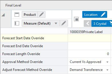
The Final Parameters view allows you to override some default measures, such as forecast method or override the approval policy. It also displays some measures that require a lower intersection than escalation level, like the plan start and end dates.
The Final Parameters view contains the following measures:
Forecast Start Date Override
This is the override of the Forecast Start Date in Basic Parameters.
If the final level is at day, and the forecast length override is specified, it can happen that the week level forecast is generated for an additional week in the future. However, when spread to day, the forecast length is respected.
The previous circumstance covers for the following case. The forecast is generated on a Tuesday, and the forecast length override 14. If a week is starting Monday, the forecast generated at week level is going to be three weeks long. However, it is going to be spread to day for only the desired 14 days.
Forecast Length Override
This is the override of the Forecast Length in Basic Parameters.
Forecast End Date Override
This is the override of the Forecast End Date in Basic Parameters.
Adjust Forecast Method Override
This is the override of the Adjust Forecast Method in Advanced Parameters .
Approval Method Override
Set only at the final-level, the Approval Method Override is a list from which you select the approval policy for individual product/location combinations. The options are:
No Override
The default approval policy is used
Manual
The system-generated forecast is not automatically approved. Forecast values must be manually approved by accessing and amending the Forecast Review view
Automatic
The system-generated quantity is automatically approved as is.
By Alert
This list of values may also include any Forecast Approval alerts that have been configured for use in the forecast approval process. Alerts are configured during the implementation and can be enabled to be used for Forecast Approval in the Enable Alert for Forecast Approval view. Refer to the Oracle Retail Predictive Application Server Configuration Tools User Guide for more information on the Alert Manager. The Alert Parameters view contains a list and descriptions of available alerts, and for which level (causal/baseline) that they are designed for.
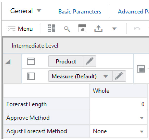
It allows you to view and set high level information, but below the global settings. For instance, you can select the approval policy or determine the history length used to calculate base demand.
The Intermediate Level view contains the following measures:
Forecast Length
The Forecast Length is used with the Forecast Start Date to determine forecast horizon. The forecast length is based on the calendar dimension of the final-level. For example, if the forecast length is to be 10 weeks, the setting for a final-level at day is 70 (10 x 7 days).
If the final level is at day, and the forecast length override is specified, it can happen that the week level forecast is generated for an additional week in the future. However, when spread to day, the forecast length is respected.
The previous circumstance covers for the following case. The forecast is generated on a Tuesday, and the forecast length override 14. If a week is starting Monday, the forecast generated at week level is going to be three weeks long. However, it is going to be spread to day for only the desired 14 days.
Approve Method
This field is a list from which you select the default automatic approval policy for forecast items. Valid values are:
Manual
The system-generated forecast is not automatically approved. Forecast values must be manually approved by accessing and amending the Forecast Review view.
Automatic
The system-generated quantity is automatically approved as is.
By Alert
This list of values may also include any Forecast Approval alerts that have been configured for use in the forecast approval process. Alerts are configured during the implementation and can be enabled to be used for Forecast Approval in the Enable Alert for Forecast Approval view. Refer to the Oracle Retail Predictive Application Server Configuration Tools User Guide for more information on the Alert Manager. The Alert Parameters view contains a list and descriptions of available alerts, and for which level (causal/baseline) that they are designed for.
Adjust Forecast Method
This measure allows you to automatically adjust the system generated forecast.
The options are:
No Adjustment
No adjustment is made to the system generated forecast
Keep Last Change
If any adjustments were done to the forecast in the previous runs, they are reflected in the Adjusted Forecast measure. In this use case, the total forecast is retained.
Keep Last Baseline
If any adjustments were done in the Adjusted Baseline in the previous runs, they are retained. In this use case. the system calculated peaks are applied on the Adjusted Baseline
Keep Last Peak
If any adjustments were done in the Adjusted Peak measure in the previous runs, they are retained. In this use case, the adjusted peaks are applied on the system calculated baseline.
Demand Transference
If Demand Transference is enabled in the plug-ins, and the necessary data is interfaced to RDFCS, and significant demand transference effects are detected, this options incorporates demand transference effects in the adjusted forecast. If demand transference effects are not zero, the system and adjusted forecasts will be different.
|
Note: The Demand Transference effects are calculated outside RDFCS. A good candidate is ORASE, the Oracle Retail science platform |
|
Note: Tables (UNKNOWN STEP NUMBER) , (UNKNOWN STEP NUMBER) , and (UNKNOWN STEP NUMBER) provide details for measure calculations for options selected in Forecast Setup. |
The available views are:
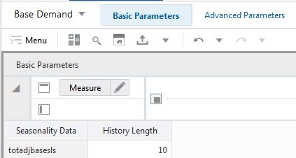
The Basic Parameters view allows you to view and set high level information for calculating base demand.
The Basic Parameters view contains the following measures:
Seasonality Data Source
This measure displays the name of the data source used to create seasonality curves.
History Length
The value entered in this field determines how many data points looking back from today are used to generate base demand.
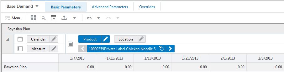
The Bayesian Plan view allows you to view and also manually change a Bayesian plan measure.
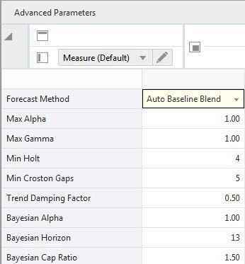
The Advanced Parameters view allows you to view a Base Demand - Advanced Parameters measure.
The Advanced Parameters view contains the following measures:
Forecast Method
This measure is a complete list of available forecast methods available to generate base demand. A summary of methods is provided in White paper.
Max Alpha
In the Simple or Holt (TrendES) model-fitting procedure, alpha (a model parameter capturing the level) is determined by optimizing the fit over the time series. This field displays the maximum value (cap value) of alpha allowed in the model-fitting process.
An alpha cap value closer to one (1) allows, but does not guarantee, more reactive models (alpha = 1, repeats the last data point). An alpha cap closer to zero (0) only allows less reactive models. The default is one (1).
The value for the optimized alpha parameter will be in the range 0.001 to Max Alpha.
Max Gamma
In the Winters (SeasonalES) and Holt (TrendES) model-fitting procedures, gamma (a model parameter capturing the trend) is determined by optimizing the fit over the time series.
Min Holt
This measure displays displays the maximum value (cap value) of gamma allowed in the model-fitting process. The value for the optimized gamma parameter will be in the range 0.001 to Max Gamma
Min Croston Gaps
The Crostons Min Gaps is the default minimum number of transitions from non-zero sales to zero sales. Thus, if Croston's Min Gap is set to five, then the method may fit if you have five or more transitions from non-zero sales to zero sales.
If there are not enough gaps between sales in a given product's sales history, the Croston's model is not considered a valid candidate model.
The system default is five minimum gaps between intermittent sales. The value must be set based on the calendar dimension of the level. For example, if the value is to be 5 weeks, the setting for a final-level at day is 35 (5x7days) and a source-level at week is 5.
Trend Damping Factor
This measure determines how reactive the forecast is to trending data. A value close to zero (0) is a high damping, while a value if one (1) implies no damping. The default is 0.5.
Bayesian Alpha
When using the Bayesian forecasting method, historic data is combined with a known sales plan in creating the forecast. As POS data comes in, a Bayesian forecast is adjusted so that the plan's magnitude is a weighted average between the original plan's scale and the scale reflected by known history
This measure displays the value of alpha (the weighted combination parameter). An alpha value closer to one (or infinity) weights the sales plan more in creating the forecast, whereas alpha closer to zero (0) weights the known history more. The default is one (1).
Bayesian Horizon
This measure determines for how many periods in the forecast horizon Bayesian formula is applied. For the rest of the forecast horizon the forecast is equal to the plan.
Let's assume the Bayesian Horizon is set to 3, and the forecast horizon is 10 periods. Then the first 3 periods of the forecast horizon the forecast is the combination of the plan and recent sales, as defined by the Bayesian formula. For the remaining 7 periods, the forecast equals the plan. If the Bayesian Horizon is set to 0 or a negative number, the Bayesian formula is used for the entire forecast horizon.
Bayesian Cap Ratio
This measure is used to cap the resulting Bayesian forecast if it deviates significantly from the sale plan. The Bayesian Cap ratio is used as follows:
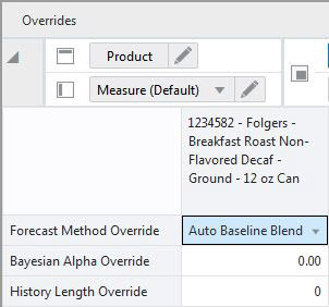
The Final Level View allows you to view a Base Demand - Final measure.
The Final Level View contains the following measures:
Forecast Method Override
Set at the final the Forecast Method Override is a list from which you can select a different forecast method to generate base demand.
No Override appears in this field if the system default is to be used.
Bayesian Alpha Override
This is the override of the Bayesian Alpha parameter that is specified in the Advanced Parameters sub-step.
An alpha value closer to one (or infinity) weights the sales plan more in creating the forecast, whereas alpha closer to zero (0) weights the known history more. The default is one (1).
History Length Override
This is the override of the History Length parameters that is specified in the Basic Parameter sub-step.
The value entered in this field determines how many data points looking back from today are used to generate base demand.
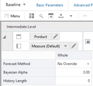
It allows you to view and set high level information, but below the global settings. For instance, you can select the approval policy or determine the history length used to calculate base demand.
The Intermediate Level view contains the following measures:
Forecast Method Override
Set at the final the Forecast Method Override is a list from which you can select a different forecast method to generate base demand.
No Override appears in this field if the system default is to be used.
Bayesian Alpha Override
This is the override of the Bayesian Alpha parameter that is specified in the Advanced Parameters sub-step.
An alpha value closer to one (or infinity) weights the sales plan more in creating the forecast, whereas alpha closer to zero (0) weights the known history more. The default is one (1).
History Length Override
This is the override of the History Length parameters that is specified in the Basic Parameter sub-step.
The value entered in this field determines how many data points looking back from today are used to generate base demand.
The available views are:
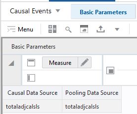
The Basic Parameters view displays the data sources used to calculate causal effects at the final and pooling levels.
The Basic Parameters view contains the following measures:
Causal Data Source
This measure displays the name of the data source used to calculate promotion effects at the final level.
Pooling Data Source
This measure displays the name of the data source used to calculate promotion effects at the pooling levels. The measure may be different than the causal data source, because at the pooling levels the data source can be normalized, something that is not recommended for the final level.
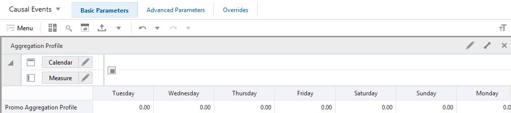
The Aggregation Profile view allows you to view and edit a day of week profile. The profile can be used to aggregate events from the day to the week level.
The Aggregation Profile view contains the following measures:
Promo Aggregation Profile
Used only for Daily Promotions, the Promo Aggregation Profile is the measure name of the profile used to aggregate promotions defined at day up to the week. The value entered in this field is the measure name of profile. Note that the only aggregation of promotion variables being performed here is along the Calendar hierarchy. RDF Cloud Service does not support aggregation of promotion variables along other hierarchies such as product and location hierarchies.
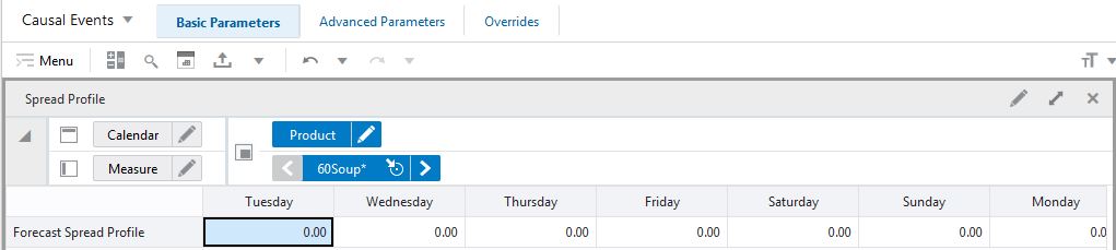
The Spread Profile view allows you to view and edit a day of week profile. The profile can be used to spread week level forecast to day.
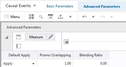
The Advanced Parameters view gives access to causal-related information that is accessed less frequently.
The Advanced Parameters view contains the following measures:
Default Apply Causal
In this measure the user specifies if promotion effects are applied on top of the baseline or not. The choices are:
Apply
Promotion effects are applied
Do Not Apply
Promotion effects are not applied
Promo Overlapping Factor
This adjustment factor specifies at a high level how the individually calculated promotions interact with each other when they are overlapping in the forecast horizon. This parameter serves as a global setting, but can be overridden at lower levels. The default value is 1.
A value greater than 1 means the promotion effects will be compressed when applied in the model, instead of linearly summing up to get the total promotion effect. The larger the value is, the larger the compression effect will be, meaning the smaller the total effect will be.
A value between 0 and 1 means the promotion effects will be amplified when applied in the model, instead of linearly summing up to get the total promotion effect. The smaller the value is, the larger the amplification effect will be, meaning the larger the total effect will be.
Blending Ratio
This parameter sets the weights for combining the Final and Pooling Level promotion effects, when calculating the blended effect. The range of the parameter is 0 to 1. A value closer to 1 will yield a blended effect closer to the Pooling Level effect. A value closer to zero yields an effect closer to the Final Level effect.
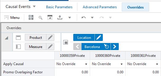
The Final view allows you to override at a more granular level some default measures related to promotions and promotion effects.
The Final view contains the following measures:
Apply Causal
In this measure the user can override the default behavior around applying promotion effects on top of the baseline or not. The choices are:
No Override
Default behavior is applied
Apply
Promotion effects are applied
Do not Apply
Promotion effects are not applied
Promo Overlapping Factor
This adjustment factor specifies at the product/location level how the individually calculated promotions interact with each other when they are overlapping in the forecast horizon. The default value is 0, meaning no override.
A value greater than 1 means the promotion effects will be compressed when applied in the model, instead of linearly summing up to get the total promotion effect. The larger the value is, the larger the compression effect will be, meaning the smaller the total effect will be.
A value between 0 and 1 means the promotion effects will be amplified when applied in the model, instead of linearly summing up to get the total promotion effect. The smaller the value is, the larger the amplification effect will be, meaning the larger the total effect will be.
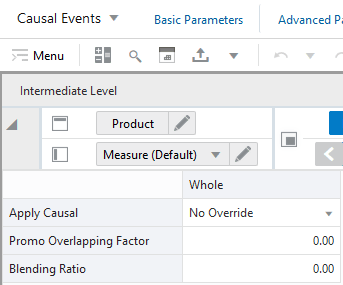
It allows you to view and set high level information, but below the global settings. For instance, you can select the approval policy or determine the history length used to calculate base demand.
The Intermediate Level view contains the following measures:
Apply Causal
In this measure, you can override the default behavior around applying promotion effects on top of the baseline or not. The choices are:
No Override
Default behavior is applied
Apply
Promotion effects are applied
Do not Apply
Promotion effects are not applied
Promo Overlapping Factor
This adjustment factor specifies at the product/location level how the individually calculated promotions interact with each other when they are overlapping in the forecast horizon. The default value is 0, meaning no override.
A value greater than 1 means the promotion effects will be compressed when applied in the model, instead of linearly summing up to get the total promotion effect. The larger the value is, the larger the compression effect will be, meaning the smaller the total effect will be.
A value between 0 and 1 means the promotion effects will be amplified when applied in the model, instead of linearly summing up to get the total promotion effect. The smaller the value is, the larger the amplification effect will be, meaning the larger the total effect will be.
Blending Ratio
This parameter sets the weights for combining the Final and Pooling Level promotion effects, when calculating the blended effect. The range of the parameter is 0 to 1. A value closer to 1 will yield a blended effect closer to the Pooling Level effect. A value closer to zero yields an effect closer to the Final Level effect. Blending the effects from pooling and final levels is combining the robustness of the effects estimated at the pooling levels with the richness of the effects estimated at the final level.
In general the pooled effects are more conservative than the final level effects. If an effect for an item/store is high, because the item is very responsive to promotions, expect its corresponding pooling effect to be less. Conversely, if an item's demand is not affected at all by promotions, you can expect the effect estimated at the pooling level to be different from zero, if other items, in the same pooling level, are responsive to promotions.
The available views are:
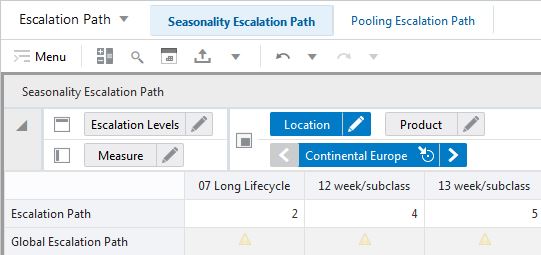
The Seasonality Escalation Path view shows the available escalation levels for long lifecycle items, and allows you to set priorities for each level.
The Seasonality Escalation Path view contains the following measures:
Seasonality Escalation Path
The user can specify the priority in which the system searches escalation levels for forecast parameters like seasonality curves and/or promotion effects. For instance, suppose there are three escalation levels available. The path may be defined as follows:
Escalation Level #1: priority 3
Escalation Level #2: priority 4
Escalation Level #3: priority 2
In this case, when generating the forecast, the system will first look to get parameters from Escalation Level #3 (highest priority). If the are available, they are used. If they are not available, because they were deemed unreliable and pruned, the system will go to Escalation Level #1 (second highest priority). Finally, if the search is not successful, the search continues at Escalation Level #2.
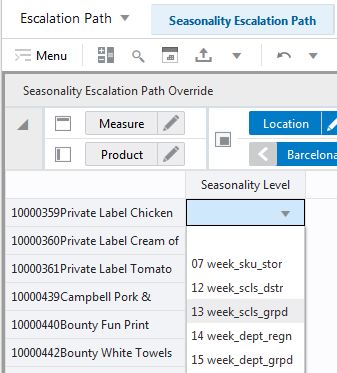
The Seasonality Escalation Path Override view allows you to choose to bypass the escalation search, by suggesting a level from which the seasonality is used.
However, if the forecast parameters for that level were deemed unreliable and pruned, the search will follow the default escalation path.
The Seasonality Escalation Path Override view contains the following measures:
Seasonality Escalation Path Override
In this field the user can override the default escalation path selections. The user can enter the preferred Escalation Level, and that will become the top priority. However, if the forecast parameters for that level were deemed unreliable and pruned, the search will follow the default escalation path.
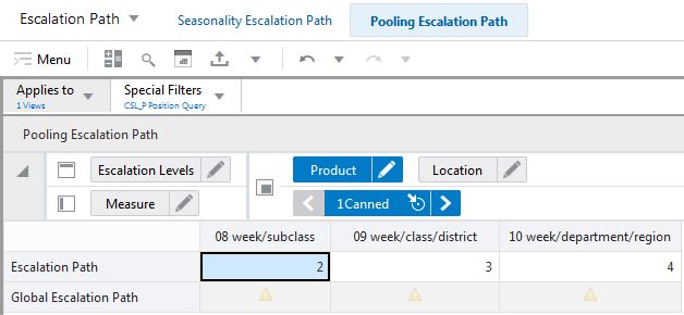
The Pooling Escalation Path view shows the available pooling levels for long lifecycle items, and allows you to set priorities for each level.
The Pooling Escalation Path view contains the following measures:
Pooling Escalation Path
The user can specify the priority in which the system searches escalation levels for forecast parameters like seasonality curves and/or promotion effects. For instance, suppose there are three escalation levels available. The path may be defined as follows:
Escalation Level #1: priority 3
Escalation Level #2: priority 4
Escalation Level #3: priority 2
In this case, when generating the forecast, the system will first look to get parameters from Escalation Level #3 (highest priority). If the are available, they are used. If they are not available, because they were deemed unreliable and pruned, the system will go to Escalation Level #1 (second highest priority). Finally, if the search is not successful, the search continues at Escalation Level #2.
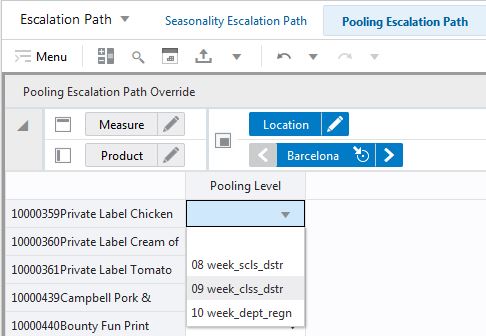
The Pooling Escalation Override Path view allows you to choose to bypass the escalation search, by suggesting a level from which the promotion effects are used.
However, if the forecast parameters for that level were deemed unreliable and pruned, the search will follow the default escalation path.
The Pooling Escalation Override Path view contains the following measures:
Pooling Escalation Override Path
In this field the user can override the default escalation path selections. She can enter the preferred Escalation Level, and that will become the top priority. However, if the forecast parameters for that level were deemed unreliable and pruned, the search will follow the default escalation path.
The available views are:
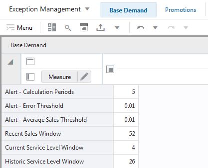
The Base Demand view allows you to view and edit threshold for exceptions relevant to baseline demand.
The Base Demand view contains the following measures:
Alert – Calculation Periods
The number stored in this field defines the number of calculations periods used in generating exceptions.
Alert – Error Threshold
This field stores the value that determines if a forecast error is acceptable, or if it needs to be flagged as exception.
Alert – Average Sales Threshold
Threshold used in deciding if average sales are high or low, depending on how they compare against the value.
Recent Sales Window
This field determines the time frame over which recent sales are considered in the exception calculations.
Current Service Level Window
This field stores the number of periods, going back from today, used to calculate the service level. This is meant to be for the current level, so the value should be something reflecting the current state. For instance the current service level could be calculated for the past week, so four or five periods.
Historic Service Level Window
This field stores the number of periods, going back from today, used to calculate the service level. This is meant to be for the historic level, so the value should be something reflecting a longer past period. For instance the current service level could be calculated for the past year or half year, so twenty six or fifty two periods.
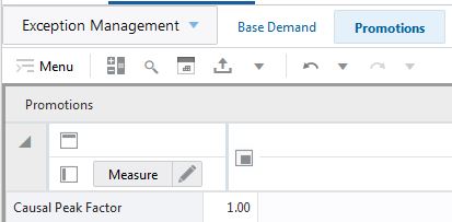
The Promotions view allows you to view and edit threshold for exceptions relevant to promotional demand.
The Promotions view contains the following measures:
Causal Peak Factor
This measure is relevant for promotional forecasting. The current forecast values are divided by the maximum historical demand. If the result is larger than the value of this measure, the forecast may be too large and an exception is triggered.
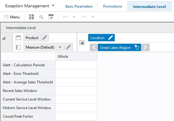
The Intermediate Level view allows you to view and edit the threshold for exceptions that are relevant to baseline and promotional demand at a more granular level than the other two views; Base Demand View and Promotions View.
The Intermediate Level View contains the following measures:
Alert – Average Sales Threshold
Threshold used in deciding if average sales are high or low, depending on how they compare against the value.
Alert – Calculation Periods
The number stored in this field defines the number of calculations periods used in generating exceptions.
Alert – Error Threshold
This field stores the value that determines if a forecast error is acceptable, or if it needs to be flagged as exception.
Causal Peak Factor
This measure is relevant for promotional forecasting. The current forecast values are divided by the maximum historical demand. If the result is larger than the value of this measure, the forecast may be too large and an exception is triggered.
Current Service Level Window
This field stores the number of periods, going back from today, used to calculate the service level. This is meant to be for the current level, so the value should be something reflecting the current state. For instance the current service level could be calculated for the past week, so four or five periods.
Historic Service Level Window
This field stores the number of periods, going back from today, used to calculate the service level. This is meant to be for the historic level, so the value should be something reflecting a longer past period. For instance the current service level could be calculated for the past year or half year, so twenty six or fifty two periods.
Recent Sales Window
This field determines the time frame over which recent sales are considered in the exception calculations.