| Oracle® Retail Demand Forecasting Cloud Service User Guide Release 19.0 F24922-17 |
|

 Previous |
 Next |
| Oracle® Retail Demand Forecasting Cloud Service User Guide Release 19.0 F24922-17 |
|
Previous |
Next |
Oracle Retail Demand Forecasting Cloud Service (RDFCS) provides accurate forecasts that enable retailers to coordinate demand-driven outcomes that deliver connected customer interactions. With a single view of demand, RDFCS provides pervasive value across retail processes, including driving optimal strategies in planning, increasing inventory productivity in supply chains, decreasing operational costs and driving customer satisfaction from engagement to sale to fulfillment. RDFCS is a comprehensive solution that maximizes the forecast accuracy for the entire product lifecycle, with tailored approaches for short and long lifecycle products, the ability to adapt to recent trends, seasonality, out-of-stocks and promotions, and reflect the unique demand drivers of each retailer. Today's progressive retail organizations know that store-level demand drives the supply chain. The ability to forecast consumer demand productively and accurately is vital to a retailer's success. The business requirements for consumer responsiveness mandate a forecasting system that more accurately forecasts at the point of sale, handles difficult demand patterns, forecasts promotions and other causal events, processes large numbers of forecasts, and minimizes the cost of human and computer resources.Forecasting drives the business tasks of planning, replenishment, purchasing, and allocation. As forecasts become more accurate, businesses run more efficiently by buying the right inventory at the right time. This ultimately lowers inventory levels, improves safety stock requirements, improves customer service, and increases the company's profitability.
A number of challenges affect the ability of forecast demand accurately including:
Overcoming Data Sparsity through Escalation and Pooling Levels
Managing Forecasting Results Through Automated Exception Reporting
Incorporating the Effects of Promotions and Other Event-Based Challenges on Demand
One challenge to accurate forecasting is the selection of the best model to account for level, trending, seasonal, and spiky demand. Oracle Retail's automatic evaluation of several methods eliminates this complexity. The automated approach can pick the best fit method among a large selection, like Simple Exponential Smoothing, Holt Exponential Smoothing, Additive and Multiplicative Winters Exponential Smoothing, Croston's Intermittent Demand Model, and Seasonal Regression forecasting.
Another approach is to combine the output of the competing methods to create a more robust forecast and minimize the risk of overfitting.
Demand at low levels, such as item/store, is usually too noisy to identify clear selling patterns, both for baseline and promotional sales. In such cases, generating a reliable forecast requires analyzing historical data at a higher level (escalation or pooling levels) in the hierarchy in which demand patterns can be consistently detected. The forecasting components estimated at these high levels, like seasonality curves and promotion effects, are combined with low level information, like base demand and trend, to create the low level forecast that is needed to drive the supply chain.
RDFCS also forecasts demand for new products and locations for which no sales history exists. There are several options for new products. First, there is the option to go on auto mode, and the user does not have to do anything. Another option is model the new product's demand based on that of an existing similar product for which you do have a history. The existing item selection can be automatically done by matching item attributes. There is also the option to manually select the item. Forecasts for the new products are copied from one item or can be a combination of multiple items. The level for the new products are copied from Like Item, the seasonal curve, and the promotional effects are from escalation.
The RDFCS end user is typically responsible for managing the forecast results for thousands of items, at hundreds of stores, across many weeks at a time. The Oracle Retail Predictive Application Server Cloud Edition (RPAS CE) platform provides users with an automated exception reporting process that indicates to you where a forecast value may lie above or below an established threshold, thereby reducing the level of interaction needed from you. The framework for exception management is implemented using multiple features.First there is the exception dashboard profile, where the user can filter down to desired merchandise/locations to view a hit count and the variance from the desired value of the forecast. Based on that information, the user can launch in a workspace where she can review only the exceptions inside the product and location's space defined in the dashboard filter settings.Once in the workspace, the user navigates to flagged positions using the workspace alerts which are synchronized with the exception dashboards. When an exception is resolved, the result is committed to the domain, and the dashboard exception count— upon refresh—reflects the change.
Promotions, non-regular holidays, and other causal events create another significant challenge to accurate forecasting. Promotions such as advertised sales and free gifts with purchase might have a significant impact on a product's sales history, as can fluctuating holidays such as Easter. The causal forecasting functionality estimates the effects that such events have on demand. The results are used to predict future sales when conditions in the selling environment are similar. This type of advanced forecasting identifies the behavioral relationship of the variable you want to forecast (sales) to both its own past and explanatory variables such as promotion and advertising.Suppose that your company has a large promotional event during the Back To School season each year. The exact date of Back To School varies from year to year; as a result, the standard time-series forecasting model often has difficulty representing this effect in the seasonal profile. The Promotional Forecasting module allows you to identify the Back To School season in all years of your sales history, and then define the upcoming Back To School date. By doing so, you can causally forecast the Back To School-related demand pattern shift.
What is Demand Transference?
When New Items are added to a retailer's assortment, the existing items' demand may be negatively impacted. Conversely, if items are removed from an assortment, the remaining items may experience a boost in demand, because there is less competition. We call this demand transference due to assortment changes.
Demand transference across items in an assortment is a challenge for all retailers. How one item effects the performance of another is difficult to predict, and can significantly impact an assortments performance overall.
Enabling demand transference in RDFCS adds to the already extensive capabilities to create more accurate and robust forecasts by incorporating the impact of assortment changes. Accurate forecasts translate to high service levels and fewer lost sales, which in turn means better margin and improved customer satisfaction. With this release, RDFCS is enhanced to layer the demand transference impact on top of the base demand, trend, seasonality, as well as price and promo information, to create a holistic version of the forecast.
Short lifecycle items have the unique trait that they sell for a relatively short period of time and then never again. This type of merchandise can be divided as fashion items, and items that have replacements. For fashion items, the demand is modeled based on items that started selling around the same time of year in the past years. For instance, a spring collection for this coming year, is modeled based on a Spring collection that started selling in February in the past year. The items that replace other items are treated differently. The demand for an item that will start selling is going to be modeled after the demand of the item that it is replacing.
For the majority of retailers, the business is managed using a calendar (364 days organized into 13 week quarters) that periodically includes an extra 53rd week so that the year end stays in about the same time of the year. It is useful to have some control over how this 53rd week will be managed within the forecasting system's time dimension. Management of this issue causes customers the pain, time and cost of configuring their data every few years that this happens.
The problem described has two implications. The first case is when two years—each with 52 weeks—of historical sales are available, and the retailer needs to forecast for the following year, which has 53 weeks. In this case, the retailer needs to have a forecast for that period, but also preserving the seasonality for the other periods. The second case is when one of the years of historical sales has 52 weeks, and the other has 53 weeks. In this case, the retailer needs to have a forecast where the 53 week history is mapped to 52 seasonality indices. There is a third case, when the 53rd week is outside the dates considered for the forecast generation. If this is the case, nothing needs to be done.
There is no special setup for handling the 53rd week. It is only the calendar file that has 53 fiscal weeks in one of the years If the 53rd week is in history, the value for that week is not taken into account when calculating time-phased metrics. Specifically for seasonality, the sales of the 53rd week are not used to calculate the 52 seasonal indices. However, for the base demand calculation, which does not have a time component, the value of the 53 week is used. If the 53rd week is in the forecast region, the seasonality for the upcoming 53rd week is the average of the week 52 and the first week of the following year.
The forecasting process represents a next generation approach engineered to provide transparency, responsiveness and accuracy through the application of retail sciences using the scale of our modern Retail Cloud Platform.
Transparency enables analytical processes and end-users to understand and engage with the forecast. This is accomplished by representing the demand model as the decomposition of intuitive components that include base rate of demand, seasonality and causal effects. The forecasting process provides transparency to the final results, individual model components and underlying decisions by the system and end-user.
Responsiveness enables the coordination and simulation of demand-driven outcomes using forecasts that adapt immediately to new information and without a dependency on batch processes. This is accomplished by separating the calculation of the forecast from the analytical processes that determine components within the forecasting model.
Accuracy enables retailers to deliver connected customer interactions while driving efficiencies to increase profits. Maximizing forecast accuracy is paramount to RDFCS. This is accomplished through the application of best-fit sciences throughout the forecasting process.
Following is a summary of the forecasting process:
Prepare Reference Data
The purpose of this step is to prepare reference data for subsequent estimation, pruning and escalation processes. The emphasis in the preparation processes is to treat anomalies in historical data, such as out-of-stock, outliers and promotions, where the objective is to increase reliability of the reference data. For long-lifecycle items where data tends to be reliable over long time periods, the anomalies are corrected. For short-lifecycle items where data tends to be unreliable over short periods, the anomalies are omitted.
Estimated Demand Parameters
The purpose of this step is to estimate all demand parameters and at all possible escalation levels. An escalation level represents a grouping of items and locations for robust parameter estimation to overcome sparsity and sensitivity. Escalation levels can be tied to explicit hierarchy levels (for example, subclass/region) or flexible item/location groupings (for example, optimized analytical clusters). As each demand parameter is estimated, multiple machine learning methods are applied, individually optimized and evaluated for accuracy. The final model can represent the best-fit method or a robust method calculated as an intelligent blending of multiple methods weighted by accuracy.
Prune
The purpose of this step is to prune escalation levels that do not pass analytical quality checks. These include data, estimation and correlation quality checks. The result is a candidate pool of high quality parameter estimates for the escalation process.
Escalate
The purpose of this step is to select the demand parameter estimate for each component of the forecast model using the candidate pool of escalation levels. The escalation process reflects the optimal balance of richness and reliability.
Forecast
The purpose of this step is to calculate the forecast through the application of demand parameter estimates from the analytical processes in conjunction with the known demand drivers and user-overrides. The demand model is completely responsive to changes in demand drivers and updates to the demand model itself (for example, user-defined override). This step also includes support for responsive new-item forecasting, with tailored approaches for new-item scenarios, such as dynamic, repeatable and similar assortments.
The user experience is delivered on our experience-inspired RPAS Cloud Edition (RPAS CE) user interface (UI). RPAS CE provides end-users with a next generation cloud-native UI that is purpose-built to accelerate intent into action for planners and forecasters. This includes interactive and visual dashboards to assess priorities, responsive and flexible workspaces to implement decisions and a coordinated exceptions framework that ties business process all the way from dashboard to cell.
The business process is engineered to maximize the productivity of end-users through exception-driven processes and emphasis on workflow simplification. The day-in-the-life processes begin with dashboard views that enable the end-user to assess the effectiveness and quality of their forecasts and prioritize exceptions. From the dashboards, the end-user is able to contextually launch into the appropriate workspace. For exception-driven processes, the end-user is guided to the point-of-resolution, with visibility to progress and the ability to iteratively work through forecasting priorities throughout the day.
The dashboard views and workspaces that support day-in-the-life forecasting workflows are summarized as follows:
Forecast Overview Dashboard
This dashboard leads with Key Performance Indicators (KPIs) that provide macro-level insight into forecasting priorities and the effectiveness of the forecasts in driving demand-driven outcomes. This enables end-users to assess forecasting complexity drivers, such as frequent promotions, and forecasting performance towards business objectives, such as fill rates.
Forecast Scorecard Dashboard
This dashboard provides insight to forecast accuracy (for example, MAPE, Bias) along with clear visibility to system performance and the impact of end-user contributions to the forecasting process. This enables forecast analysts and managers to identify forecast process improvement priorities.
Exception Dashboards
The exception dashboards represent the primary starting point for day-in-the-life processes. The short and long lifecycle forecasting processes each have a dedicated dashboard that enables end-users to efficiently drive decisions through focused exception-driven processes. From here, end-users are able to define the scope of exceptions to be managed through dashboard filters and launch directly to workspace views tailored for resolution. As exceptions are resolved, the dashboard is updated to enable end-users to iteratively work through forecasting priorities.
Forecast Review Workspaces
The forecast approval workspaces represent the primary point of interaction with the demand forecasts. The short and long lifecycle forecasting processes each have a dedicated forecast approval workspace to enable end-users to efficiently review, adjust, and approve their forecasts. This is supported by a rich set of decision support metrics and the ability to responsively simulate forecast updates based on new demand drivers and different forecasting methods. The workspace also features real-time alerts and dedicate exception management views that navigate end-users to the point resolution.
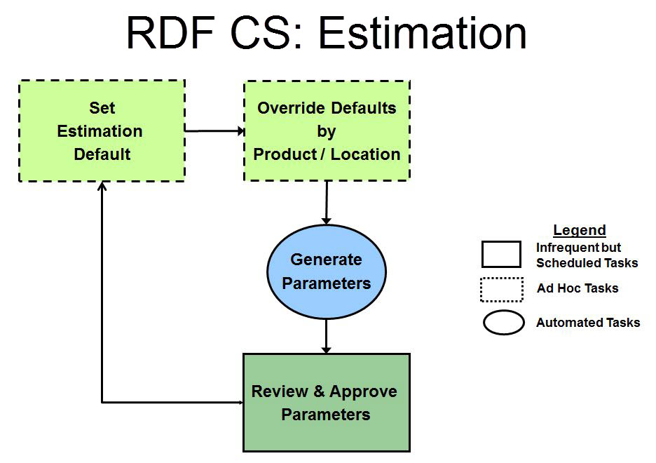
Not visible to the end user is the forecast engine, and all the tasks happening behind the scenes. The batch is split between estimation and forecasting. Estimation consists of the heavy data mining of historical demand to generate the necessary forecast parameters like seasonality, price and promo effects. Following are tasks which comprise the estimation workflow.
After estimation is run, the forecast parameters are computed, and everything is available to generate the forecast. Since most metrics are already pre-calculated during estimation, this step is very quick, allowing for extensive What-if in the Forecast review workspace. Following are the tasks related to generating, reviewing, and approving forecasts.