Understanding Cubes
The key concept of online analytical processing (OLAP) is that of a cube. In this document, we use the term cube to refer to any analytic data store. An OLAP cube is a collection of related data—a database—that has multiple dimensions. The term cube dimensions roughly describes the equivalent of fields in a relational database. In terms of data analysis, dimensions can be thought of as criteria—such as time, account, and salesperson—that can pinpoint a particular piece of data. These pieces of data are usually transactions from an online transaction processing (OLTP) system.
Although they are called cubes, OLAP databases can have more than three dimensions. In fact, most cubes have three to eight dimensions. To understand the concept of OLAP cubes, start with a simple data analysis model and then expand it.
Suppose you want to analyze unit sales of your company. You can examine the total units that were sold in a particular year, but that number might not help you understand much about your business. Instead, you might want to see unit sales broken down by time and by product. The matrix that you use to analyze this data might look like the following table, which represents a cube with two dimensions (time and product).
|
Product |
2001 |
2002 |
2003 |
|---|---|---|---|
|
Widgets |
3000 |
6500 |
8200 |
|
Gadgets |
1200 |
1450 |
3000 |
|
Doohickeys |
2500 |
3400 |
2000 |
|
Whatzits |
500 |
670 |
1300 |
Dimensions and Members
In OLAP terminology, the preceding table is an OLAP cube that represents units sold dimensioned by time and product. Time and product are the dimensions of the cube, and units sold is the fact data.
In the preceding table, each dimension is subdivided into categories, called cube members, which represent individual years and products.
In the time dimension, the members are 2001, 2002, and 2003.
In the product dimension, the members are widgets, gadgets, doohickeys, and whatzits.
Measures and Cells
In the preceding table, the values of the most interest are not years or products. The purpose of the table is to find the number of units that were sold. Sold units make up the data element that is being evaluated or measured. In OLAP terminology, the number of units sold is called the measure, or fact, of this cube. The areas of the table where members intersect with other members represent individual measure and fact values. These intersections are called cells. The italicized cell in the preceding table represents the number of widgets sold in 2002: 6500 units.
Multiple Dimensions
The two-dimensional cube represented by the table in the Understanding Cubes section is basic for reporting purposes. For example, it does not provide data about where any of the units were sold. You can provide this information by adding another dimension, location, to the model, as shown in the following diagram.
Image: Diagram of a cube with three dimensions
This diagram illustrates a cube with three dimensions.
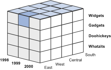
The preceding three-dimensional OLAP cube represents units sold dimensioned by time, product, and location. (The location members are East, West, Central, and South.) The shaded cell represents the number of widgets sold in the East region in 1999. You could find the number of units sold for any other product in any other region at any other time by finding the cell at the intersection point of three members, one from each dimension.
Suppose you also want to factor customer accounts into the analysis. Although showing four dimensions graphically is a challenge, the result of this added dimension is clear: in our example, each cell of the OLAP cube represents the intersection of an account, a year, a region, and a product.
Hierarchy is the organization of cube data elements with their reporting structures. It represents both the hierarchy and the method of consolidation in a dimension level.
The example cube has only one level in each dimension. The time dimension consists of one level containing three members (years), and the location dimension consists of one level containing four members (regions). However, the data used to build such OLAP cubes probably supports more than just one level in each dimension.
For example, when a company records a sale, that sale occurs in a particular month, which occurs in a particular quarter and in a particular year. You can examine the time dimension at one of three levels: month, quarter, or year. Likewise, you can record that each sale occurs in a particular office, in a particular city, or in a particular region. The location dimension might also have three levels, such as office, city, and region.
As mentioned, the categories found at each level of a dimension are called members. You can envision multilevel dimensions as tree diagrams, the members of which relate to each other in various parent-child relationships. Some members are parents of other members, some are children, and some are both.
Image: Example of a time hierarchy diagram
This diagram shows an example of a portion of a typical time dimension with its various levels and members.
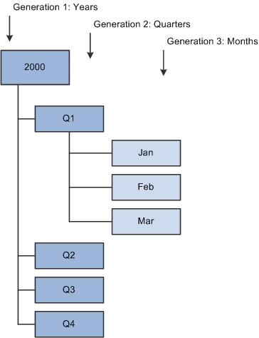
Each box in the diagram represents a unique member. This diagram is familiar to PeopleSoft Tree Manager users. In fact, PeopleSoft trees can play an important role in defining the hierarchy of an OLAP cube.
See PeopleSoft Tree Manager Overview.
Consolidation
Viewing the dimension of a hierarchy tells you about the organization of its members, but you should consider another facet of the dimension. You need to know how to consolidate the values that are found under child members into the value of their parent members. For example, the children might be added together to equal the parent. This scenario is certainly the case in a time dimension, in which the value for each member is added to its siblings to equal the value of its parent. (Three months can be consolidated into their parent quarter, four quarters can be consolidated into their parent year, and so on.)
The following table shows the cube example, adding a second level, quarters, to the time dimension of the original example.
Image: Consolidation example in tabular format
This table shows the cube example, adding a second level, quarters, to the time dimension of the original example.
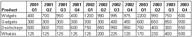
To consolidate the data
at the quarterly level into the yearly level, the quarterly data is
added together. The 2001 rollup is Q1 2001 + Q2 2001 + Q3
2001 + Q4 2001.
However, you also might find dimensions in which certain members are to be subtracted from their siblings, such as in a profit dimension. In such a dimension, suppose two members are at the first level, margin and total expenses, both of which are reported as positive values. To find the total profits, you would not add margin and total expenses, instead you would subtract total expenses from margin.