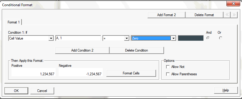
Applying Formatting to Auto Calculated Data Rows and Columns

You can use the conditional formatting feature to apply additional formatting to the auto calculation rows and columns, such as underline, bold, and indent. The conditional formatting feature contains two conditions specifically designed for auto calculation:

Auto Calculation—Used to apply formatting to the auto calculated cells and auto calculation heading.
Auto Calculation Group Heading—Used to apply formatting to the section headings.

For more information on conditional formatting, see Applying Conditional Formatting to Grids.

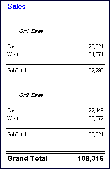
Figure 3, Print Preview of Example Report with Applied Conditional Formatting, displayed below, is an example report that uses conditional formatting to specify font, alignment, and border and shading settings. The following conditions were applied to the example report by selecting the East, West Heading Cell and Calculated Data Cell:

Format 1: IF (Auto Calculation Year is True, then Format Cells (double border top, Font = Ariel, Bold, Font size = 12)
Format 2: IF (Auto Calculation Market is True, then Format Cells (single border top)
Format 3: IF (Auto Calculation Group Heading Market is True, then Format Cells (Alignment = center, Font Style = italic)
Format 4: IF (Auto Calculation Group Heading Year is True, then Format Cells (Bold, Font size = 12, Color = blue)
Figure 3. Print Preview of Example Report with Applied Conditional Formatting

To apply formatting to calculated data rows and columns:

Open a report.
Select a cell or group of cells that is set up with auto calculation.
Select Format, and then Conditional Format.
Select Auto Calculation or Auto Calculation Group Heading from the Property drop-down list located below Condition 1: If, then enter the conditions.
Figure 4. Conditional Formatting Applied to Specify an Auto Calculated Cell
Click the Format Cells button to apply formatting to the calculated cell.
Click OK to accept the formatting than you specified for the calculated cell. For more information on formatting, see Formatting Grids.
Note:
You can use conditional formatting to establish formatting for calculated cells. For more information, see Applying Conditional Formatting to Grids.
To view the report, select File, and then Print Preview. The example report resembles Figure 3, Print Preview of Example Report with Applied Conditional Formatting.