Multiple Subject Areas in a Single Analytic
This topic discusses how to use multiple subject areas in a single analysis.
Subject areas can be tricky to master, but once you get familiar with them you can easily mix and match subject area components for your analytics. The reason you would want to do this is just for flexibility. You might want to look at your business from different perspectives.
You can create an analysis that combines attributes and metrics from custom permit and standard permit-related subject areas that share a common dimension. Or, if that isn't enough, you can create an analysis that combines data from multiple standard subject areas.
To start with, let's learn how to add a subject area to the editing palette. Whether you're creating a new analysis, or using an existing analysis to add objects from your custom subject area, the steps for adding multiple custom or standard subject areas to your palette are the same.
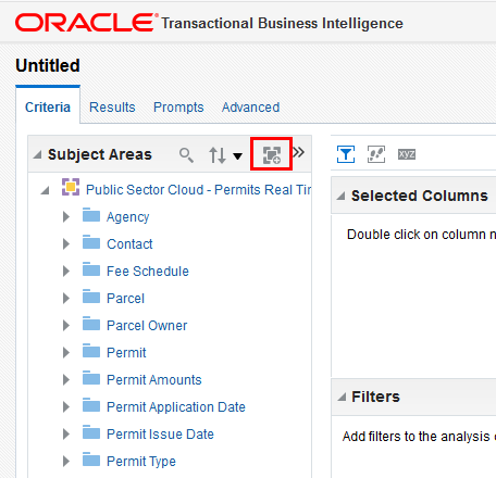
To add multiple subject areas to editing palettes:
Create your analysis using a single subject area.
In the Subject Areas section, click the Add / Remove Subject Areas icon.
This shows the Add / Remove Subject Areas icon.
Select or remove one or more standard or custom subject areas from this analysis by selecting or deselecting subject area. If you have created custom subject areas, they also appear in this list under the name you assigned to them.
Cross Subject Area Queries
Each subject area contains a collection of attributes and measures relating to the one-dimensional STAR model and grouped into individual folders. The term STAR refers to the semantic model where a single fact is joined to multiple dimensions. You can create an analysis that combines data from more than one subject area. This type of analysis is referred to as a cross-subject area query. Cross-subject area queries are classified into three broad categories:
Combining queries from multiple subject areas.
Using common (conformed) dimensions.
Using local and common (conformed) dimensions.
Using a “set” operation (Union or Union All, for example) to combine more than one result set from different subject areas.
Combining Logical SQL using the Advanced tab.
A common dimension is a dimension that exists in all subject areas that are being joined in an analysis. For example, the Contact dimension is the common dimension for the Public Sector Cloud - Permit Inspection Activity Real Time and Public Sector Cloud - Permits Real Time subject areas.
A local dimension is a dimension that exists only in one subject area. For example, Inspection Type and Inspection Status are local dimensions for the Public Sector Cloud - Permit Inspection Activity Real Time subject area.
The following are some general guidelines to follow when working with multiple subject areas:
If all metrics and attributes needed for the analysis are available in a single subject area and fact metrics, use that subject area only and don't create a cross-subject area query. Such an analysis performs better and is easier to maintain.
When joining two subject areas in an analysis, make sure at least one attribute from a common dimension is used in the analysis.
When using common dimensions always choose attributes from the common dimension from a single subject area. For instance if you're using the Contact dimension to build a query between subject area 1 and subject area 2, then select all Contact dimension attributes from either subject area 1 or from subject area 2. (Not some contact attributes from subject area 1 and some from subject area 2.) In some scenarios, the common dimension may have more attributes in one subject area than the other. In such a situation, you can only use the subset of common attributes for a cross-subject area query.
Always include a measure from each subject area that's being used in your analysis. You don't have to display measures or use them, but you should include them. You can hide a measure if not needed in the analysis.
When using common and local dimensions use SET VARIABLE ENABLE_DIMENSIONALITY=1; in the Advanced SQL tab.
Queries from Multiple Subject Areas
The simplest and fastest way to generate an analysis is to use a single subject area. If the dimension attributes and fact metrics that you're interested in are all available from a single subject area, then you should use that subject area to build the analysis. Such an analysis results in better performance and is much easier to maintain.
If your analysis requirements can't be met by any single subject area because you need metrics from more than one subject area, you can build a cross-subject area query using common dimensions. There's a clear advantage to building a cross-subject area query using only common dimensions, which is recommended.
Keep in mind that if you use three subject areas for an analysis, your common dimensions must exist in all three subject areas. Joining on common dimensions gives you the benefit of including any metric from any of the subject areas in a single analysis.
While you can create an analysis joining any subject area to which you have access, only a cross-subject area query that uses common dimensions returns data that's at the same dimension grain. This happens so that the data is cleanly merged and the result is an analysis that returns exactly the data you want to see.
Knowing how cross-subject area queries are executed in BI helps you understand the importance of using common dimensions when building such an analysis. When a cross-subject area analysis is generated, separate queries are executed for each subject area in the analysis and the results are merged to generate the final analysis. The data that's returned from the different subject areas is merged using the common dimensions. When you use common dimensions, the result set returned by each subject area query is at the same dimensional grain, so it can be cleanly merged and rendered in the analysis.
Common Dimensions for an Analysis
Here is an example of combining common dimensions. In this case, we combine the Permit Count, Permit Type, Inspection Count, and Inspection District Type. The common dimension in both subject areas used for this analysis is Permit Type and different fact metrics are pulled from each subject area.
The following subject areas are used for this example analysis:
Subject area 1: “Public Sector Cloud – Permits Real Time”
Subject area 2: “Public Sector Cloud – Permit Inspection Activity Real Time”
Customer is the common dimension used for this example analysis:
“Public Sector Cloud – Permits Real Time”.“Permit Type” – Permit Type
“Public Sector Cloud – Permit Inspection Activity Real Time“ – Permit Type
The following are the metric measures for this example analysis:
“Public Sector Cloud – Permits Real Time“.“Permit Amounts” – Permit Count
“Public Sector Cloud – Permit Inspection Activity Real Time“.“Inspection Amounts” – Inspection Count
Local and Common Dimensions for an Analysis
This example pulls the Permit Count by Permit Type and Inspection Count by Inspection District Type. Permit Type is a common dimension in both subject areas used for this query. Inspection District is a local dimension to the Public Sector Cloud – Permit Inspection Activity Real Time subject area. Different fact metrics are pulled from each subject area. Note that use of local dimension may impact the grain of the analysis. In such cases the metrics may get repeated for each of these rows.
The following are the subject areas used for this example analysis:
Subject area 1: “Public Sector Cloud – Permits Real Time”
Subject area 2: “Public Sector Cloud – Permit Inspection Activity Real Time”
Permit Type is the common dimension for this example analysis: “Public Sector Cloud – Permits Real Time”.“Permit Type” – Permit Type.
The following is the local dimensions used for this example analysis: “Public Sector Cloud - Permit Inspection Activity Real Time”.“Inspection District” – Inspection District.
The following are the metrics (measures) used for this analysis:
“Public Sector Cloud – Permits Real Time”.“Permit Amounts” – Permit Count
“Public Sector Cloud – Permit Inspection Activity Real Time“.“Inspection Amounts” – Inspection Count
The following is the logical SQL used for this analysis:
SET VARIABLE ENABLE_DIMENSIONALITY=1;SELECT

   0 s_0,

   "Public Sector Cloud - Permits Real Time"."Permit Type"."Permit Type" s_1,

   "Public Sector Cloud - Permit Inspection Activity Real Time"."Inspection District"."District Type" s_2,

   "Public Sector Cloud - Permits Real Time"."Permit Amounts"."Permit Count" s_3,

   "Public Sector Cloud - Permit Inspection Activity Real Time"."Inspection Amounts"."Inspection Count" s_4

FROM "Public Sector Cloud - Permits Real Time"

ORDER BY 1, 2 ASC NULLS LAST, 3 ASC NULLS LAST

FETCH FIRST 75001 ROWS ONLY
Set Operations to Combine Result Sets from a Subject Area
This example creates a compound analysis query that's a union of two result subsets from two subject areas, combining results from:
Permit Count by Permit Type from the Public Sector Cloud – Permits Real Time subject area (result 1)
Inspection Count by Inspection District from the Public Sector Cloud - Permit Inspection Activity Real Time subject area (result 2)
SELECT saw_0, saw_1 FROM ((SELECT 'Permits ~ ' ||"Permit Type"."Permit Type" saw_0, "Permit Amounts"."Permit Count" saw_1 FROM "Public Sector Cloud -  Permits Real Time")
UNION
(SELECT 'Inspection ~ ' ||"Inspection District"."District Id" saw_0, "Inspection Amounts"."Inspection Count" saw_1 FROM "Public Sector Cloud - Permit Inspection Activity Real Time")) t1 ORDER BY saw_0
Logical SQL Using the Advanced Tab
If your requirement can't be met by either of the two methods already discussed, then there's another advanced technique you can try. This technique lets you join multiple logical SQL statements based on common IDs or keys, which can be written against the same or different subject areas, just as used in normal SQL. Both Outer and Equijoin are supported.
This example illustrates how you can combine Permits and Fees data in an analysis by combining the logical SQL found on the Advanced tab.
Step 1: Write a BI Answers query using the “Public Sector Cloud – Permits Real Time” subject area to show the Fee amount and Applicant Name. Once the correct results are achieved, go to the Advanced tab and grab the logical SQL associated with this query.
Logical SQL for Query 1:
SELECT
   0 s_0,
   "Public Sector Cloud - Permits Real Time"."Applicant"."Applicant Name" s_1,
   "Public Sector Cloud - Permits Real Time"."Permit"."Permit Number" Per_No,
   "Public Sector Cloud - Permits Real Time"."Permit Amounts"."Fee Amount" s_3
FROM "Public Sector Cloud - Permits Real Time"
Step 2: Write a second BI Answers query using the " Public Sector Cloud - Receipts Real Time"."Transactions" subject area to show fees paid for the permit. Once the correct results are achieved, go to the Advanced tab and grab the logical SQL associated with this query.
Logical SQL for Query 2:
SELECT
   0 s_0,
   "Public Sector Cloud - Receipts Real Time"."Transactions"."Application ID" s_1,
   "Public Sector Cloud - Receipts Real Time"."Fact - Receipts"."Amount Received for a given period" s_2
FROM "Public Sector Cloud - Receipts Real Time"
Step 3: Go to the Advanced tab in BI Answers and copy/paste the following logical SQL which is an OBIEE - Equijoin of the two previous SQL statements based on Opportunity ID. Use any text editor to combine the logical SQL statements copied from Steps 1 and 2.
SELECT
permit.s_1, permit.Per_No, permit.s_3, fees.s_2
FROM
(
SELECT
   0 s_0,
   "Public Sector Cloud - Permits Real Time"."Applicant"."Applicant Name" s_1,
   "Public Sector Cloud - Permits Real Time"."Permit"."Permit Number" Per_No,
   "Public Sector Cloud - Permits Real Time"."Permit Amounts"."Fee Amount" s_3
FROM "Public Sector Cloud - Permits Real Time"
) permit,
(
SELECT
   0 s_0,
   "Public Sector Cloud - Receipts Real Time"."Transactions"."Application ID" s_1,
   "Public Sector Cloud - Receipts Real Time"."Fact - Receipts"."Amount Received for a given period" s_2
FROM "Public Sector Cloud - Receipts Real Time"
) fees
WHERE permit.Per_No = fees.s_1 Custom and Standard Subject Areas Joins
Analyses can be build using combinations of standard, as well as both custom and standard subject areas. The add subject area option appears once you have created an analysis from a single subject area. You can delete subject areas using these same steps. When you create your analysis, you select a single subject area during the creation steps. Once the analysis is created, you add additional standard or custom subject areas.