Use Fair-Share Rules to Allocate Scarce Supply

In many industries, when supply is constrained at the source locations, the replenishment plans allocate available inventory proportionally among competing demand locations. You can now allocate scarce supply to competing demand locations by first meeting sales-order demand and then proportionally fulfilling inventory-level needs so that all demand locations progress toward their inventory targets at comparable rates.

Bottom-up visibility exposes downstream demand at the source, and unmet demand rolls forward from bucket to bucket so that priority and fairness are preserved. You can monitor the allocation using new measures for clear, auditable outcomes. This update results in fair-share allocation across the supply network, reduced stockouts at critical nodes, and consistent execution of replenishment policies.

To enable fair-share allocation, select the checkbox named Enable fair-share allocation in the Advanced supply options step in the Redwood guided process for creating or editing your multiechelon replenishment plan.

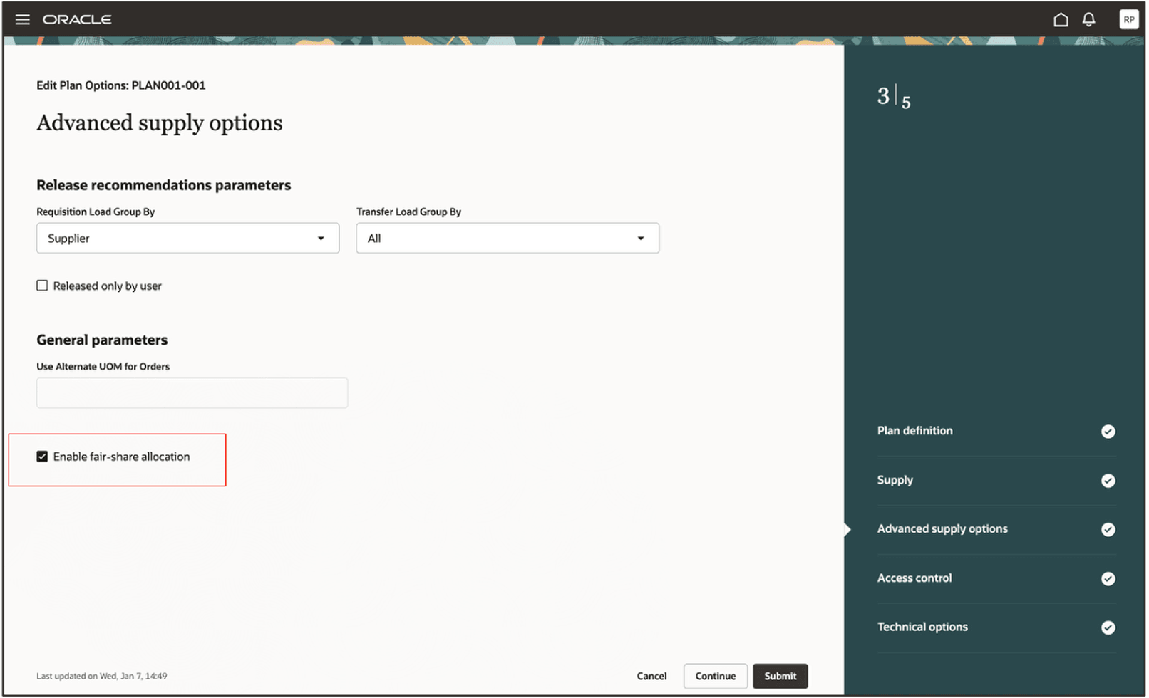
Advanced Supply Options Step in Redwood Guided Process for Creating or Editing Multiechelon Replenishment Plan

High-Level Summary of Fair-Share Allocation

These points provide a high-level summary of how fair-share allocation of supplies is accomplished for multiechelon replenishment plans:

• The goal is to proportionately allocate scarce supply at a source location to competing demand locations by first allocating supply to sales-order demand across all locations and then fulfilling inventory-level needs so that all demand locations progress toward their inventory targets at comparable rates.
• For achieving this objective, source locations are provided with visibility of customer demands at destination locations. During the bottom-up pass, for every replenishment recommendation (unconstrained planned order), the breakup of sales-order demand and inventory-level demand is provided to each source location.
• During the top-down pass, the constrained supply at the source is first allocated to demands for transfer orders, movement requests, and firm planned orders because supplies are already committed for these demands.
• The next priority is given to sales-order demands. The constrained supplies are proportionately allocated to sales-order demands of competing locations.
• Inventory-level demands of competing locations are then met proportionately with the remaining supply. This arrangement implies that all bands within the inventory-level demands (minimum level, safety stock level and maximum level) including forecast demands are brought to the same proportionate levels. The fulfillment of the forecast, safety stock, and minimum and maximum levels aren’t separately tracked.
• The unmet demands of the previous time bucket are added to the demand of the current bucket, and then the total demand competes for a fair share of the supply in the order of the demand types.
• To summarize, demands are met in the following order:
  1. Transfer orders, movement requests, and firm planned orders
  2. Local sales orders and downstream sales orders
  3. Inventory-level demand and downstream inventory-level demand

• The fair-share allocation results can be reviewed with the new measures listed later in this write-up.

Examples

Consider a supply chain that has a distribution center named D1 and two stores named S1 and S2. All the locations participate in the fair-share allocation.

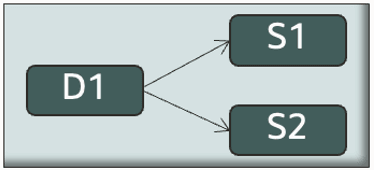
Supply Chain for Fair-Share Allocation

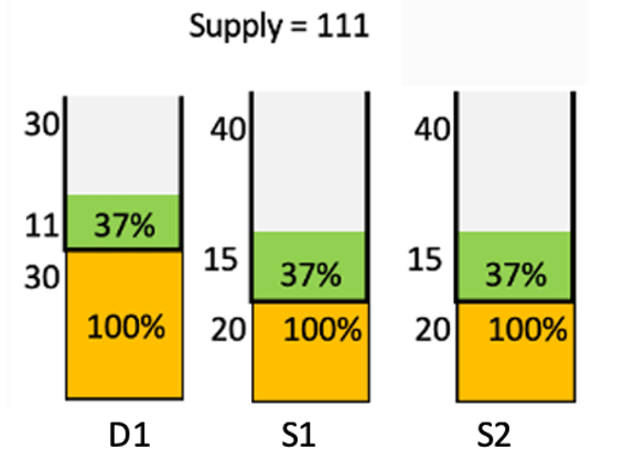
The details of the first example are as follows:

• Available supply at D1: 111 units
• Inventory-level demand at each location: 60:60:60
• Supply allocated at each location: 37:37:37
• Allocation percentage for inventory-level demand: 61:61:61
• Outcome:
  • Planned order of 37 units from D1 to S1
  • Planned order of 37 units from D1 to S2

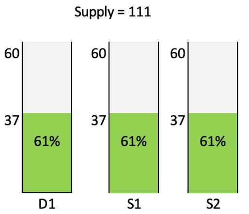
First Example for Fair-Share Allocation

The details of the second example are as follows:

• Available supply at D1: 110 units
• Sales orders at D1: 30 units
• Sales orders at S1 and S2: zero units
• Inventory-level demand at each location: 30:60:60
• Allocation percentage for sales orders at D1: 100
• Units after allocation for sales orders at D1: 80 units
• Supply allocated at each location: 16:32:32
• Allocation percentage for inventory-level demand: 53:53:53
• Outcome:
  • Planned order of 32 units from D1 to S1
  • Planned order of 32 units from D1 to S2

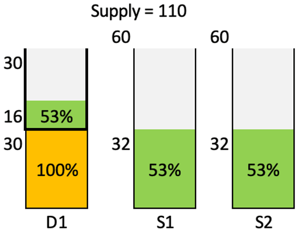
Second Example for Fair-Share Allocation

The details of the third example are as follows:

• Available supply at D1: 111 units
• Sales orders at D1, S1, and S2: 30:20:20
• Inventory-level demand at each location: 30:40:40
• Allocation percentage for sales orders: 100:100:100
• Units after allocation for sales orders: 41 units
• Supply allocated at each location: 11:15:15
• Allocation percentage for inventory-level demand: 37:37:37
• Outcome:
  • Planned order of 35 units from D1 to S1 (20 units for sales-order demand and 15 units for inventory-level demand)
  • Planned order of 35 units from D1 to S2 (20 units for sales-order demand and 15 units for inventory-level demand)

Third Example for Fair-Share Allocation

New Measures for Fair-Share Allocation

This table provides details about the newly-added measures for fair-share allocation:

Name	Description	Comment
Cumulative Effective Supply for Allocation	Cumulative effective supply available for allocation at the start of a given time bucket at an item-location combination. The supply also includes unused supply from the previous time bucket.
Local Sales Order Demand	Local sales-order demand for an item-location combination.	The measure includes sales orders from the current order date for unconstrained planned orders until one day before the next order date for unconstrained planned orders.
Allocated Quantity for Local Sales Order Demand	Allocated quantity for the local sales-order demand for an item-location combination.
Local Inventory Demand	Local inventory-level demand for an item-location combination.
Allocated Quantity for Local Inventory Demand	Allocated quantity for the local inventory-level demand for an item-location combination.
Downstream Sales Order Demand	Sales-order demand for an item at a downstream location.
Allocated Quantity for Downstream Sales Order Demand	Allocated quantity for the sales-order demand for an item at a downstream location.
Downstream Inventory Demand	Inventory-level demand for an item at a downstream location.
Allocated Quantity for Downstream Inventory Demand	Allocated quantity for the inventory-level demand for an item at a downstream location.
Achieved Coverage of Outbound Sales Order Demand	Percentage of coverage achieved for the outbound sales-order demand for an item-location combination.	Outbound sales-order demand includes local sales-order demand and downstream sales-order demand. The measure is calculated as follows: [(Allocated Quantity for Local Sales Order Demand + Allocated Quantity for Downstream Sales Order Demand)/(Local Sales Order Demand + Downstream Sales Order Demand)] * 100
Achieved Coverage of Outbound Inventory Demand	Percentage of coverage achieved for the outbound inventory-level demand for an item-location combination.	Outbound inventory-level demand includes local inventory-level demand and downstream inventory-level demand. The measure is calculated as follows: [(Allocated Quantity for Local Inventory Demand + Allocated Quantity for Downstream Inventory Demand)/(Local Inventory Demand + Downstream Inventory Demand)] * 100
Inbound Sales Order Requirement	Quantity that needs to be allocated for the inbound sales-order demand for an item-location combination after netting of the supplies.	This quantity needs to be allocated from an upstream location for the netted sales-order demand for an item at a downstream location.
Achieved Requirement for Inbound Sales Orders	Allocated quantity for the achieved requirement for inbound sales orders for an item at a downstream location.
Achieved Coverage of Requirement for Inbound Sales Orders	Percentage of coverage achieved for the requirement of inbound sales orders for an item at a downstream location.	The measure is calculated as follows: [(Achieved Requirement for Inbound Sales Orders)/(Inbound Sales Order Requirement)] * 100
Inbound Inventory Requirement	Quantity that needs to be allocated from an upstream location for the inbound inventory requirement for an item at a downstream location.
Achieved Requirement for Inbound Inventory	Allocated quantity for the achieved requirement for inbound inventory for an item at a downstream location.
Achieved Coverage of Requirement for Inbound Inventory	Percentage of coverage achieved for the requirement of inbound inventory for an item at a downstream location.	The measure is calculated as follows: [(Achieved Requirement for Inbound Inventory)/(Inbound Inventory Requirement)] * 100
Effective Supply for Allocation	Effective supply available at the start of a given day for allocation at an item-location combination.

These measures are in the Inventory Analysis measure catalog.

Detailed Example

Consider a supply chain that has a distribution center named D1 and two stores named S1 and S2. The lead time for an order from D1 to S1 or S2 is three days.

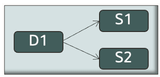
Supply Chain for Fair-Share Allocation

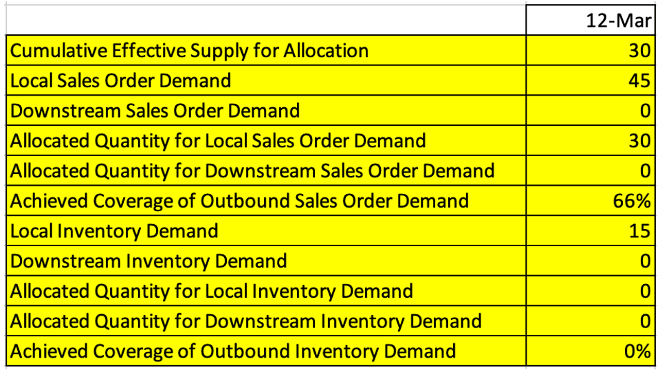
• At S1, during the unconstrained, bottom-up pass for multiechelon replenishment planning, for every replenishment recommendation (unconstrained planned order), the portion of sales-order demand and inventory-level demand is calculated.
  • The value of the Local Sales Order Demand measure is 45 units, which is sum of all the sales orders until one day before the next order date for unconstrained planned orders.
  • The value of the Downstream Sales Order Demand measure is zero units because S1 is the furthest downstream in the supply chain.
  • The value of the Inbound Sales Order Requirement measure is calculated as Local Sales Order Demand – any available supplies until March 15 (one day before the next unconstrained planned order) + any demands until March 15. In this case, the value will be 15 units (45–30 (On Hand measure)). The sales order demand that is percolated to the upstream node is netted first with the existing supplies.
  • The value of the Local Inventory Demand measure is calculated as 15 units (Replenishment order quantity–Local Sales Order Demand–Downstream Sales Order Demand, 60–45–0).
  • The value of the Inbound Inventory Requirement measure is calculated as 45 units (Replenishment order quantity–Inbound Sales Order Requirement, 60–15).

The following figure depicts the demand and supply for S1 during the bottom-up pass:

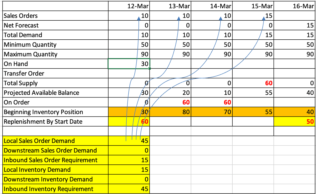
Demand and Supply for S1 During Bottom-Up Pass

• Let’s assume that S2 has the same demand-and-supply picture as S1 during the bottom-up pass.
• At D1, during the unconstrained, bottom-up pass, similar calculations are done.
  • The value of the Downstream Sales Order Demand measure is 30 units, which is the sum of the values of 15 units each for S1 and S2 for the Inbound Sales Order Requirement measure.
  • The value of the Downstream Inventory Demand measure is 90 units, which is the sum of values of 45 units each for S1 and S2 for the Inbound Inventory Requirement measure.

The following figure depicts the demand and supply for D1 during the bottom-up pass:

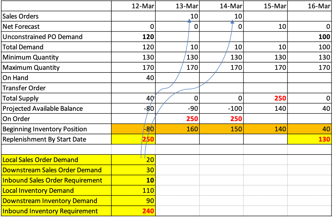
Demand and Supply for D1 During Bottom-Up Pass

• During the constrained, top-down pass at D1, the supply of 40 units on March 12 is fairly shared with the local sales-order demands of 20, 15, and 15 units at D1, S1, and S2 respectively with an allocation percentage of 80%. Note that inventory-level demand at all three locations isn’t met.

The following figure depicts the allocation at D1 during the top-down pass:

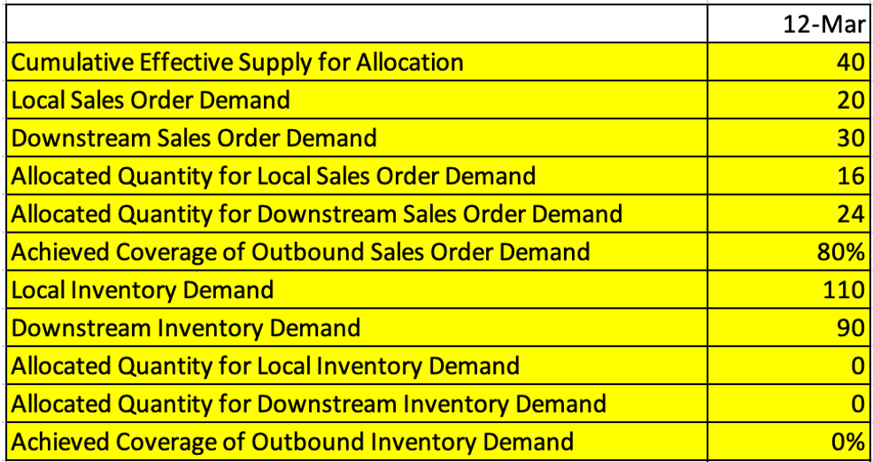
Allocation at D1 During Top-Down Pass

• Based on the value of 24 units for the measure named Allocated Quantity for Downstream Sales Order Demand at D1, the value of 12 units for the measure named Achieved Requirement for Inbound Sales Orders is calculated at S1 and S2.

The following figure depicts the measure values at S1 during the top-down pass for D1:

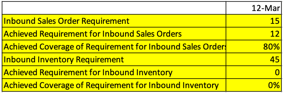
Measure Values at S1 During Top-Down Pass for D1

• During the top-down pass for D1, the measure values for S2 will be the same as those for S1.

The following figure depicts the allocation at S1 during the top-down pass:

Allocation at S1 During Top-Down Pass

• During the top-down pass, the allocation for S2 will be the same as that for S1.
• The allocated quantity of 12 units from D1 during the top-down pass will be used at S1 for allocation only after the lead time of three days and then reflected in the cumulative effective supply for allocation at S1.
• This computation is repeated for all the time buckets. Any unmet demand of a previous bucket is rolled over to the next bucket.
• Note that D1 has a buy-from sourcing rule. So, during the top-down pass at D1, the following measures are computed with the assumption that the supply is unconstrained:

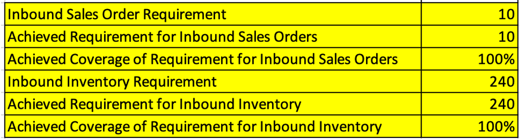
Measures Reflecting Unconstrained Incoming Supply at D1 During Top-Down Pass at D1

Steps to enable and configure

Use the Opt In UI to enable this feature. For instructions, refer to the Optional Uptake of New Features section of this document.

Offering: Supply Chain Planning

Tips and considerations

If you want to use the Use Fair-Share Rules to Allocate Scarce Supply feature, then you must opt in to its parent feature: Replenishment Planning. If you’ve already opted in to this parent feature, then you don’t have to opt in again.

• For every replenishment recommendation (unconstrained planned order), the portions of sales-order demand and inventory-level demand are calculated.
• On a day without unconstrained planned orders, the value of the Local Sales Order Demand measure will be equal to the sales orders on that day, and the value of the Local Inventory Demand measure will be equal to the forecast on that day.

For example, if the first unconstrained planned order is not on the first day of the planning horizon and is instead on Day 5, then, on each day until Day 4, the value of the Local Sales Order Demand measure will be equal to the sales orders on that day, and the value of the Local Inventory Demand measure will be equal to the forecast on that day.

• The values for the Inbound Sales Order Requirement and Inbound Inventory Requirement measures are calculated only on days when unconstrained planned orders are present. Hence, these measures have dates that are equal to the order dates of the unconstrained planned orders. The Achieved Requirement for Inbound Sales Orders and Achieved Requirement for Inbound Inventory measures will also have the same date if the demand is met on time.
• The Downstream Sales Order Demand and Downstream Inventory Demand measures at the upstream locations are populated on the ship dates of the unconstrained planned orders.
• You can quickly analyze the fair-share results by configuring a pivot table at an aggregate time level (for example, week) with the following measures:
  • Achieved Coverage of Outbound Sales Order Demand
  • Achieved Coverage of Outbound Inventory Demand
  • Achieved Coverage of Requirement for Inbound Sales Orders
  • Achieved Coverage of Requirement for Inbound Inventory

Key resources

• Introduction to Replenishment Planning Cloud (update 19D) in the readiness training
• Replenishment Planning Training on Oracle Cloud Customer Connect

Access requirements

Users who are assigned a configured job role that contains these privileges can access this feature:

• Manage Segments (MSC_MANAGE_SEGMENTS_PRIV)
• Monitor Replenishment Planning Work Area (MSC_MONITOR_REPLENISHMENT_PLANNING_WORK_AREA_PRIV)

These privileges were available prior to this update.