Solve Order in Member Formulas (Hybrid mode only)
Solve Order is a metadata property that can be set either for a dimension or a member that defines the order of member evaluation. The solve order is applied during query execution.
Solve Order can impact the performance of the query. The value of the solve order property determines the priority with which the member formula is calculated. The formula on the members that have a specified solve order are calculated in order from the lowest solve order to the highest.
You can set solve order for dimensions or members, or you can use the default Essbase solve order. The minimum solve order you can set is 0, and the maximum is 127. A higher solve order means the member is calculated later; for example, a member with a solve order of 1 is solved before a member with a solve order of 2.
Note:
This applies only for hybrid optimized applications. See: Optimizing the Application Model for Hybrid AggregationTable 15-14 Default Solve Order Settings
| Dimension/Member Type | Default Solve Order Value |
|---|---|
| Stored members | 0 |
| Sparse dimensions | 10 |
| Dense dimension - Account | 30 |
| Dense dimension - Time | 40 |
| Dense dimension | 50 |
| Attribute dimension | 90 |
| Two pass dynamic members | 100 |
In summary, the default solve order in hybrid mode dictates that stored members are calculated before dynamic calc members, and sparse dimensions are calculated before dense dimensions, in the order in which they appear in the outline (top to bottom).
Dynamic members (with or without formulas) that do not have a specified solve order inherit the solve order of their dimension unless they are tagged as two-pass. Two-pass calculation is a setting you can apply, in non-hybrid mode, to members with formulas that must be calculated twice to produce the correct value.
Two-pass is not applicable in hybrid mode, and any members tagged as two-pass are calculated last, after attributes. In hybrid mode, you should implement a custom solve order, instead of two-pass, if the default solve order does not meet your requirements.
The default solve order in hybrid mode is optimized for these scenarios:
- Forward references, in which a dynamic member formula references a member that comes later in the outline order. There is no outline order dependency in hybrid mode.
- Aggregation of child values based on outline order more closely matches aggregation using equivalent formulas.
- Dynamic dense members as dependencies inside sparse formulas. In hybrid mode, if a sparse formula references a dense dynamic member, the reference is ignored, because sparse dimensions are calculated first. To change this, assign a solve order to the sparse dimension that is higher than (calculated later than) the dense dimension’s solve order.
If you need to use a non-default solve order, you can set a custom solve order for members in hybrid mode. See Setting the Solve Order (Hybrid mode only) for how to modify solve order.
If you implement a custom solve order, it overrides the default solve order. If members or dimensions have equal solve order, the order in which they appear in the outline (top to bottom) resolves the conflict.
This behavior can be changed by assigning a custom solve order to the sparse dimension that is higher than the dense dimension’s solve order.
Example:
Consider the following example with members of different Solve Orders.
Account (Sparse, default Solve Order 30)
-
A1
-
A2
-
Ratio – Member Formula [A1 / A2]
(default Solve Order 30 inherited from Account)
Data Source (Sparse, default Solve Order 10)
-
DataInput
-
CustomInput
-
Variance – Member Formula [DataInput - CustomInput]
(default Solve Order 10 inherited from Data Source)
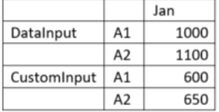
Consider the following dataset for the intersections for the January period:

Calculations with different Solve Orders for Ratio and Variance
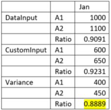
Case 1: Ratio with a higher Solve Order than Variance
In this case, Variance will be calculated first, and then corresponding Ratio.

Ratio of Variance will be calculated as (Variance->A1)/(Variance->A2).

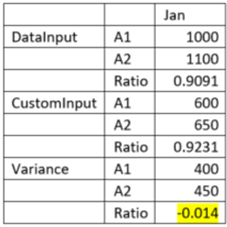
Case 2: Ratio with a lower Solve Order than Variance
In this case, Ratio will be calculated first, and then corresponding Variance.

Variance of Ratio will be calculated as (Ratio->DataInput) – (Ratio->CustomInput).
