Model Monitoring

Model monitoring allows you to monitor the quality of model predictions over time and helps you with insights on the causes of model quality issues.

The Model Monitor page allows you to create, run, and track model monitors and results. This page lists the model monitors. You can preview the model drift by selecting a single model monitor of interest, as shown in the screenshot below. In this screenshot, the monitor Power Consumption is selected. On the lower pane of the Model Monitors page, the Model Drift for the selected monitor is displayed. The X axis depicts the analysis period, and the Y axis depicts the model drift values. The horizontal red dotted line is the threshold value. The line depicts the drift value for each point in time for the analysis period. Hover your mouse over the line to view the drift values.

Figure 1: Model Monitors page

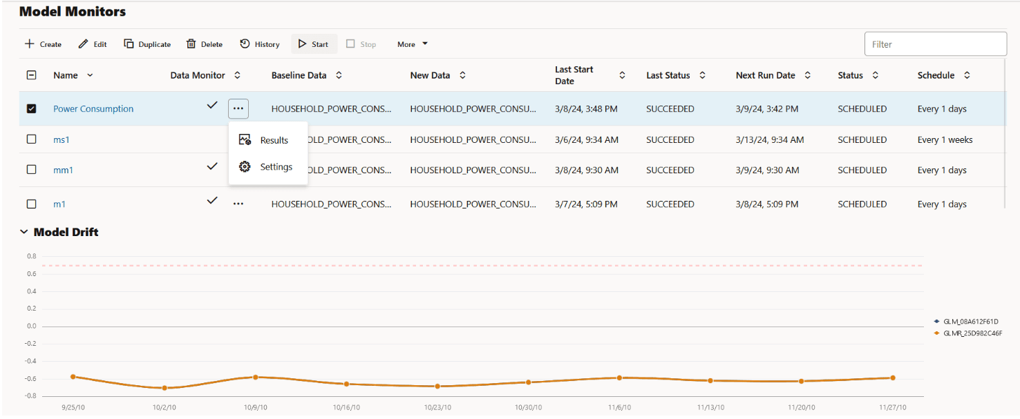
Description of the illustration model_drift_mm.png

You can perform the following tasks on the Model Monitors page:

• Create: Create a model monitor.

• Edit: Select a model monitor and click Edit to edit the monitor.

• Duplicate: Select a model monitor and click Duplicate to create a copy of the monitor.

• Delete: Select a model monitor and click Delete to delete the model monitor.

• History: Select a model monitor and click History to view the runtime details of the model monitor. If there is a data monitor job associated with the model monitor, the data monitor runtime details are displayed on the lower pane. Click Back to Monitors to go back to the Model Monitoring page.

• Start: Start a model monitor.

• Stop: Stop a model monitor that is running.

• More: Select a model monitor, click More and then click:

  • Enable: Enable a model monitor schedule. By default, the model monitor is enabled. The status is displayed as SCHEDULED.

  • Disable: Disable a model monitor schedule. The status is displayed as DISABLED.

  • Show Managed Monitors: Click this option to view the models created and managed by OML Services REST API.

The Model Monitors page displays the following information about the model monitors:

• Name: This is the name of the model monitor.

• Data Monitor: The check mark in this column indicates that there is a data monitor job associated with the model monitor. Click on the three dots to view: Figure 2: View Results and Settings of Data Monitor

  

  Description of the illustration data_monitor_options.png

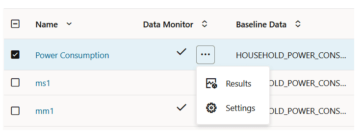
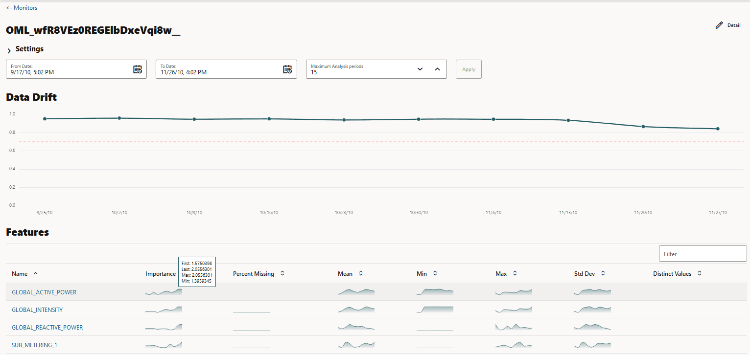
• Results: Displays the data monitoring results computed by the data monitor job. The data monitor name is auto-generated along with the prefix OML. The data drift and monitored features along with the computed statistics are displayed in view-only mode on a separate page. Click Monitors on the top left corner to return to the Model Monitors page. Click Details on the top right corner to view the settings of the data monitor. Figure 3: Data Monitor Results

  

  Description of the illustration results_dm_mm.png

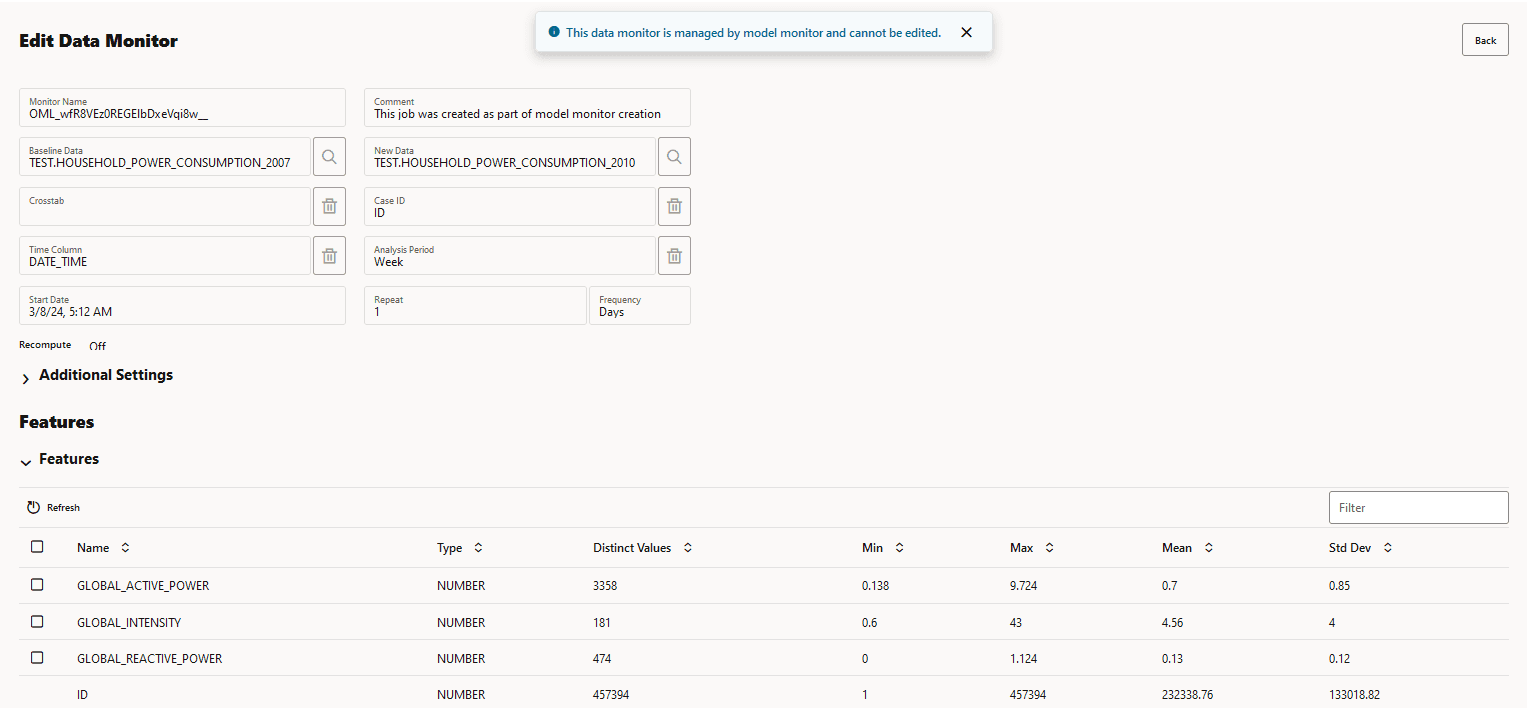
• Settings: Displays the data monitor settings, additional settings, and the monitored features in view-only mode. Click Back on the top right corner of the page to return to the Model Monitors page. Figure 4: Data Monitor Settings

  

  Description of the illustration settings_dm_mm.png

• Baseline Data: This is a table or view that contains baseline data to monitor.

• New Data: This is a table or view with new data to be compared against the baseline data.

• Last Start Date: This is the date on which the model monitor was last started.

• Last Status: This is the latest status of the model monitor. The statuses are SUCCEEDED, FAILED, RUNNING, SCHEDULED.

• Next Run Date: This is the date on which the next run is scheduled.

• Status: This is the current status of the model monitor.

• Schedule: This is the frequency of the monitoring job, that is, how frequently the model monitor is set to run on the New Data.

• Create a Model Monitor A model monitor helps you monitor several compatible models, and compute the model drift chart. Compatible models refer to those models that are trained on the same target and mining function. The model drift chart consists of multiple series of data drift points, one for each monitored model.

• View Model Monitor Results The Model Monitor Results page displays the monitoring results of each model that are being monitored. By clicking on any model that has run successfully, you can view the detailed analysis of each model such as model drift, model metrics, prediction statistics, feature impact, prediction distribution and predictive versus drift importance for each feature. The predictive impact versus drift importance for each monitored feature is computed only if data monitoring is enabled.

• View Model History The History page displays the runtime details of the model monitors.

Create a Model Monitor

A model monitor helps you monitor several compatible models, and compute the model drift chart. Compatible models refer to those models that are trained on the same target and mining function. The model drift chart consists of multiple series of data drift points, one for each monitored model.

A model monitor can optionally monitor data to provide additional insight. This additional insight is the Drift Feature Importance versus Predictive Feature Impact chart which is generated when you select the Monitor Data option while creating the model monitor.

This topic discusses hows how to create a model monitor. The example uses the Individual household electricity consumption dataset which includes various consumption metrics of a household for the year 2009. The data is split into seasons - SPRING, SUMMER, FALL, and WINTER. The goal is to understand if and how household consumption has changed over the seasons. The example shows how to track the effects of data drifts on model predictive accuracy.

The dataset comprises the following columns:

• DATE_TIME: Contains the date and time related information in dd:mm:yyyy:hh:mm:ss format.

• GLOBAL_ACTIVE_POWER: This is the household global minute-averaged active power (in kilowatt).

• GLOBAL_REACTIVE_POWER: This is the household global minute-averaged reactive power (in kilowatt).

• VOLTAGE: This is the Minute-averaged voltage (in volt).

• GLOBAL_INTENSITY: This is the household global minute-averaged current intensity (in ampere).

• SUB_METERING_1: This is the energy sub-metering No. 1 (in watt-hour of active energy). It corresponds to the kitchen.

• SUB_METERING_2: This is the energy sub-metering No. 2 (in watt-hour of active energy). It corresponds to the laundry room.

• SUB_METERING_3: This is the energy sub-metering No. 2 (in watt-hour of active energy). It corresponds to an electric water heater and air conditioner.

To create a model monitor:

1. On the Oracle Machine Learning UI left navigation menu, expand Monitoring and then click Models to open the Model Monitoring page. Alternatively, you can click on the Model Monitoring icon to open the Model Monitoring page.

2. On the Model Monitoring page, click Create to open the New Model Monitor page.

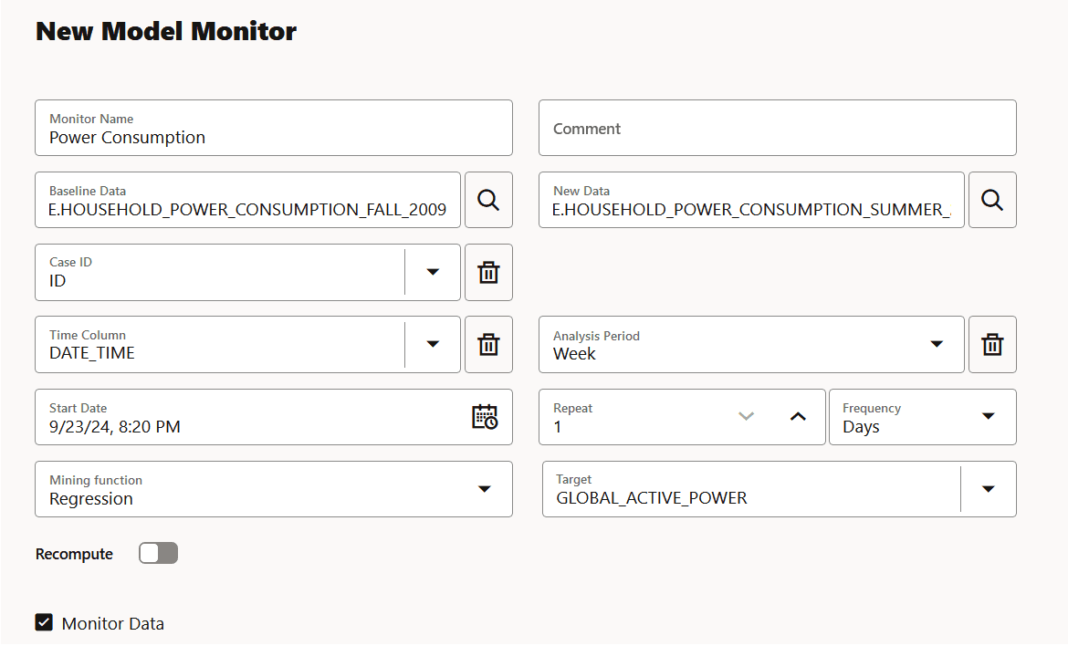
3. On the New Model Monitor page, enter the following details:

   Figure 5: New Model Monitor page

   

   Description of the illustration new_model_monitor.png

   1. Monitor Name: Enter a name for the model monitor. Here, the name Power Consumption is used.

   2. Comment: Enter comments. This is an optional field.

   3. Baseline Data: This is a table or view that contains baseline data to monitor. Click the search icon to open the Select Table dialog. Select a schema, and then a table. Here, the table containing the data for the year 2007 is selected.

   4. New Data: This is a table or view with new data to be compared against the baseline data. Click the search icon to open the Select Table dialog. Select a schema, and then a table. Here, the table containing the data for the year 2009 is selected.

   5. Case ID: This is an optional field. Enter a case identifier for the baseline and new data to improve the repeatability of the results.

   6. Time Column: This is the name of a column storing time information in the New Data table or view. The DATE_TIME column is selected from the drop-down list.

      Note: If the Time Column is blank, the entire New Data is treated as one period.

   7. Analysis Period: This is the length of time for which model monitoring is performed on the New Data. Select the analysis period for model monitoring. The options are Day, Week, Month, Year.

   8. Start Date: This is the start date of your model monitor schedule. If you do not provide a start date, the current date will be used as the start date.

   9. Repeat: This value defines the number of times the model monitor run will be repeated for the frequency defined. Enter a number between 1 and 99. For example, if you enter 2 in the Repeat field here, and Minutes in the Frequency field, then the model monitor will run every 2 minutes.

   10. Frequency: This value determines how frequently the model monitor run will be performed on the New Data. Select a frequency for model monitoring. The options are Minutes, Hours, Days, Weeks, Months. For example, if you select Minutes in the Frequency field, 2 in the Repeat field, and 5/30/23 in the Start Date field, then as per the schedule, the model monitor will run from 5/30/23 every 2 minutes.

   11. Mining Function: The available mining functions are Regression and Classification. Select a function as applicable. In this example, Regression is selected.

   12. Target: Select an attribute from the drop-down list. In this example, GLOBAL_ACTIVE_POWER is used as the target for regression models.

   13. Recompute: Select this option to update the already computed periods. This means that only time periods not present in the output result table will be computed. By default, Recompute is disabled.

   • When enabled, the drift analysis is performed for the time period specified in the Start Date field and the end time. The analysis will overwrite the already existing results for the specified time period. This means that the analysis will be computed for the time period with new data other than the current data.

   • When disabled, the data for the time period that is present in the results table will be retained as is. Only the new data for the most recent time period will be considered for analysis, and the results will be added to the results table.

     1. Monitor Data: Select this option to enable data monitoring for the specified data. When enabled, a data monitor is also created along with the model monitor to compute the Predictive Feature Impact versus Drift Feature Impact in the model specific results.

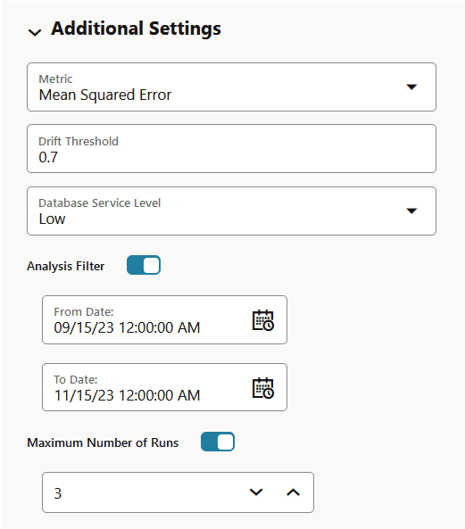
4. Click Additional Settings to expand this section and provide advanced settings for your model monitor:

   Figure 6: Additional Settings section on the New Model Monitor page

   

   Description of the illustration additional_settings_mm.png

   1. Metric: Depending on the mining function selected in the Mining Function field in the Create Model Monitor page, the applicable metrics are listed. Click on the drop-down list to select a metric.

      For the mining function Classification, the metrics are:

      • Accuracy: Calculates the proportion of correctly classifies cases - both Positive and Negative. For example, if there are a total of TP (True Positives)+TN (True Negatives) correctly classified cases out of TP+TN+FP+FN (True Positives+True Negatives+False Positives+False Negatives) cases, then the formula is:

        Accuracy = (TP+TN)/(TP+TN+FP+FN)

      • Balanced Accuracy: Evaluates how good a binary classifier is. It is especially useful when the classes are imbalanced, that is, when one of the two classes appears a lot more often than the other. This often happens in many settings such as Anomaly Detection etc.

      • ROC AUC (Area under the ROC Curve): Provides an aggregate measure of discrimination regardless of the decision threshold. AUC - ROC curve is a performance measurement for the classification problems at various threshold settings.

      • Recall: Calculates the proportion of actual Positives that is correctly classified.

      • Precision: Calculates the proportion of predicted Positives that is True Positive.

      • F1 Score: Combines precision and recall into a single number. F1-score is computed using harmonic mean which is calculated by the formula:

        F1-score = 2 × (precision × recall)/(precision + recall)

      For multi-class classification, the metrics are:

      • Accuracy

      • Balanced Accuracy

      • Macro_F1

      • Macro_Precision

      • Macro_Recall

      • Weighted_F1

      • Weighted_Precision

      • Weighted_Recall

      For Regression, the metrics are:

      • R2: A statistical measure that calculates how close the data are to the fitted regression line. In general, the higher the value of R-squared, the better the model fits your data. The value of R2 is always between 0 to 1, where:

        • 0 indicates that the model explains none of the variability of the response data around its mean.

        • 1 indicates that the model explains all the variability of the response data around its mean.

      • Mean Squared Error: This is the mean of the squared difference of predicted and true targets.

      • Mean Absolute Error: This is the mean of the absolute difference of predicted and true targets.

      • Median Absolute Error: This is the median of the absolute difference between predicted and true targets.

   2. Drift Threshold: Drift captures the relative change in performance between the baseline data and the new data period. Based on your specific machine learning problem, set the threshold value for your model drift detection. The default is 0.7.

      • A drift above this threshold indicates a significant change in model predictions. Exceeding the threshold indicates that rebuilding and redeploying your model may be necessary.

      • A drift below this threshold indicates that there are insufficient changes in the data to warrant further investigation or action.

   3. Database Service Level: This is the service level for the job, which can be LOW, MEDIUM, HIGH, or GPU.

   4. Analysis Filter: Enable this option if you want the model monitoring analysis for a specific time period. Move the slider to the right to enable it, and then select a date in From Date and To Date fields respectively. By default, this field is disabled.

      • From Date: This is the start date or timestamp of monitoring in New Data. It assumes the existence of a time column in the table. This is a mandatory field if you use the Analysis Filter option.

      • To Date: This is the end date or timestamp of monitoring in the New Data. It assumes the existence of a time column in the table. This is a mandatory field if you use the Analysis Filter option.

   5. Maximum Number of Runs: This is the maximum number of times the model monitor can be run according to this schedule. The default is 3.

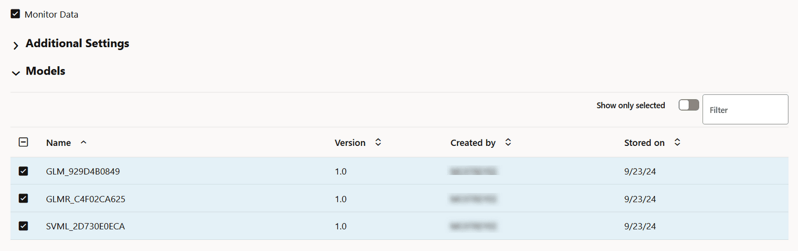
5. In the Models section, select the model that you want to monitor and then click Save on the top right corner of the page. Once you provide a value in the Mining Function and Target fields, the list of models that have been deployed are obtained and is displayed here in the Models section. Models are deployed from the Models page, or from the AutoML Leaderboard. You can view the complete list of deployed models in the Deployments tab on the Models page. The deployed models are managed by OML Services.

   Note: If you drop any models, you have to redeploy the models. Models are not schema based models, but models deployed to OML Services.

   Figure 7: Models section on the New Model Monitor page

   

   Description of the illustration models_grid.png

   Once the model monitor is successfully created, it displays the message: Model monitor has been created successfully.

   Note: You must now go to the Model Monitoring page, select the model monitor and click Start to begin model monitoring.

View Model Monitor Results

The Model Monitor Results page displays the monitoring results of each model that are being monitored. By clicking on any model that has run successfully, you can view the detailed analysis of each model such as model drift, model metrics, prediction statistics, feature impact, prediction distribution and predictive versus drift importance for each feature. The predictive impact versus drift importance for each monitored feature is computed only if data monitoring is enabled.

1. Model Monitor Results page

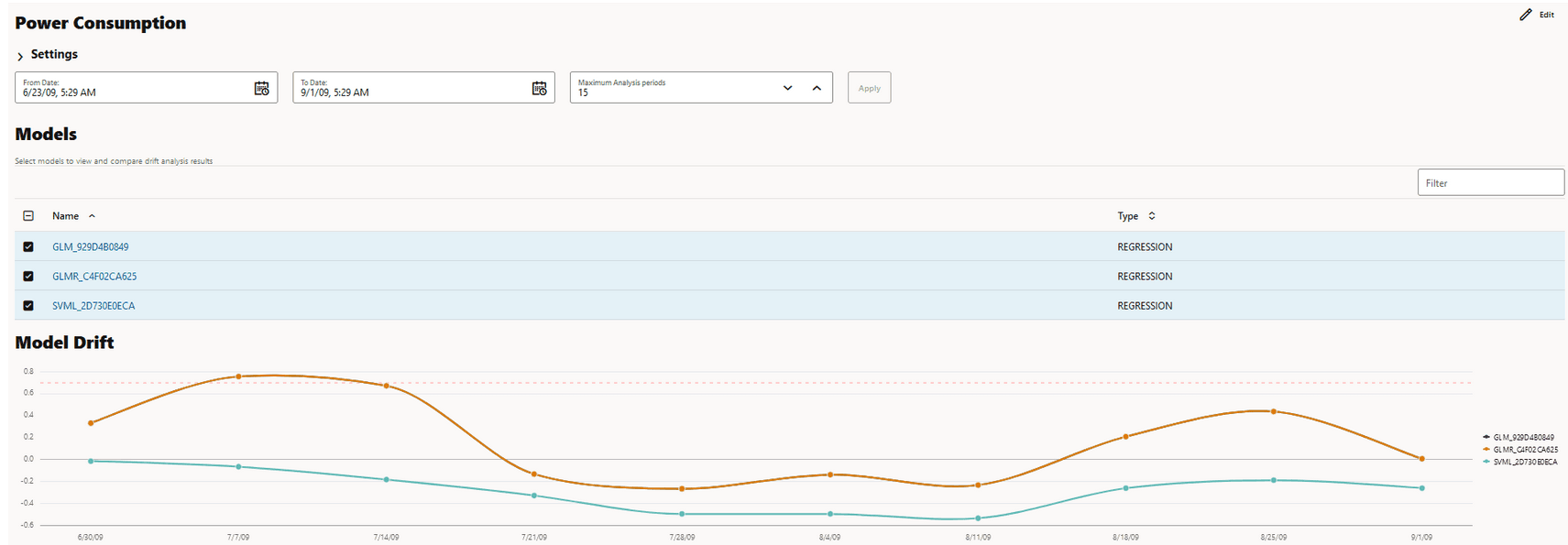
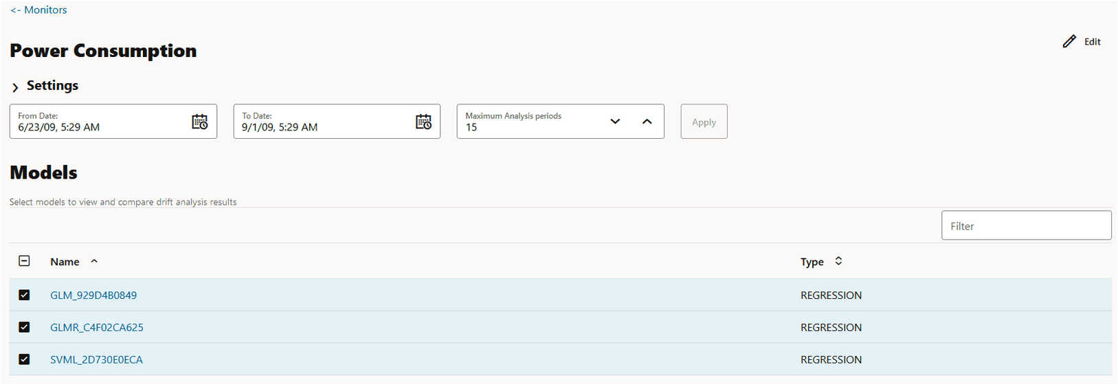
The Model Monitor Results page lists all the models that are monitored by the monitor. The name of the monitor is displayed at the top of the page. As seen in this screenshot, the monitor name Power Consumption is displayed at the top. The models GLM_929D4B0849, GLMR_C4F02CA625 and SVML_2D730E0ECA monitored by the Power Consumption monitor are listed in the Models section. By default, the details of all the monitored models are displayed. You can choose to view the details of one monitor at a time by deselecting the other monitors.

Figure 8: Model Monitor Results page

Description of the illustration model_monitor_results.png

The Model Monitor Results page comprises these sections:

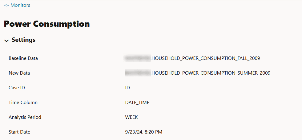
• Settings: The Settings section displays the model monitor settings. Click on the arrow against Settings to expand this section. You have the option to edit the model monitor settings by clicking Edit on the top right corner of the page.

  Figure 9: Model Monitor Settings

  

  Description of the illustration settings_section_mm.png

• Models: The Models section lists all the models that are monitored by the monitor. In this example, the models GLM_929D4B0849, GLMR_C4F02CA625 and SVML_2D730E0ECA monitored by the Power Consumption monitor are listed. Figure 10: Models on the Model Monitor Results page

  

  Description of the illustration models_mmresults.png

  You can choose to view and compare the results of one or more monitored models by deselecting the ones that you want to exclude. You can also view the results of each feature of the model by clicking on the model. These results — Feature Impact chart, Prediction Distribution, and Predictive Impact versus Drift Importance chart are displayed on a separate pane that slides in.

  Note: The Predictive Impact versus Drift Importance chart is computed only if the Monitor Data option is selected while creating the model monitor.

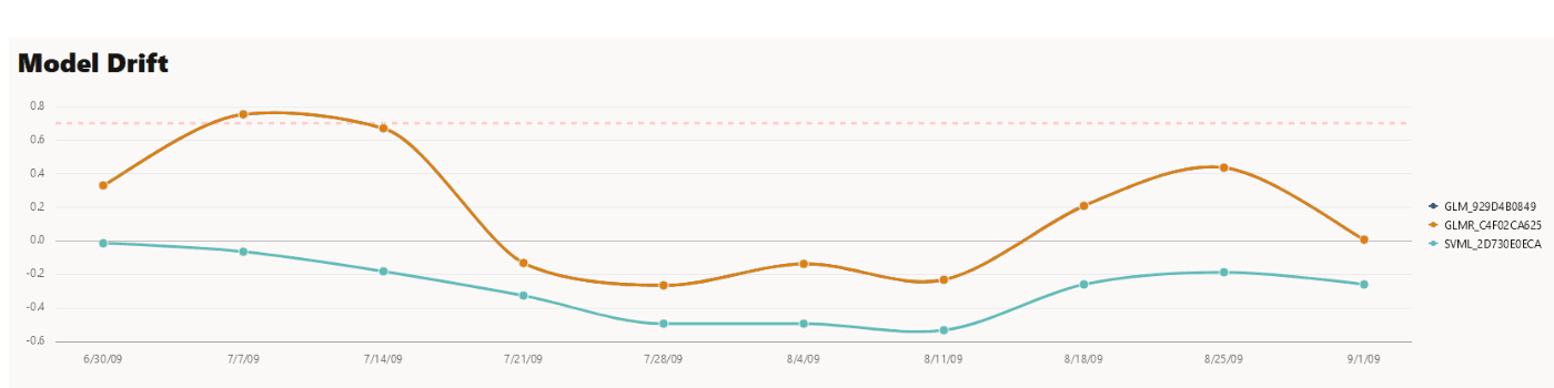
• Model Drift: The Model Drift section is displayed just below the Models section. Model drift is the percentage change in the performance metric between the baseline period and the new period. A negative value indicates that the new period has a better performance metric which could happen due to noise.

  The X axis depicts the analysis period, and the Y axis depicts the drift values. The horizontal dotted line represents the drift threshold settings that each monitor gets by default. The default covers the typical use case. However, you can choose to customize it based on specific use case. The line depicts the drift value for each point in time for the analysis period. Hover your mouse over the line to view the drift values. A drift above the threshold indicates significant change in model predictions. Exceeding the threshold suggests rebuilding and redeploying your model may be necessary. If the drift is below the threshold, it indicates that there are insufficient changes in the data to warrant further investigation or action. That is, possibly rebuilding a machine learning model using this data.

  Figure 11: Model Drift on the Models Monitor Results page

  

  Description of the illustration modeldrift_mmresults.png

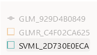
  If you want to view the drift details of one model at a time, click on the model name on the right to select or deselect it, as shown here.

  

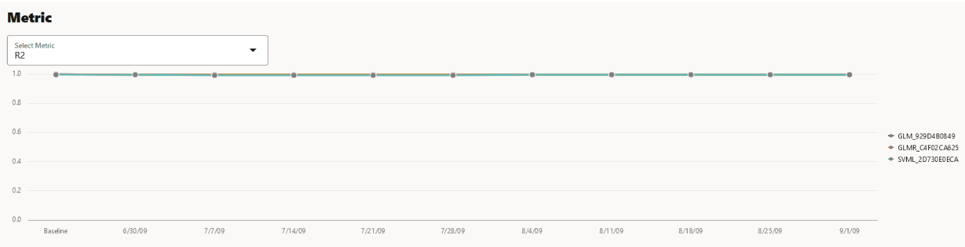
• Metric: This Metric section displays the computed metrics for the selected models. The computed metric is plotted along the y axis, and the time period is plotted along the x axis. In this example, the metric R2 or R-squared is displayed for all the three models. Hover your cursor on other points on the line to view the details of the computed metric. The value of R2 for all the models is equal to 1. Here, the value of R2 for all the three monitored models is 1. This indicates that all the three models are good fit for the data.

  Figure 12: Metric

  

  Description of the illustration model_details2.png

  The computed metrics for Regression are:

  • R2: A statistical measure that calculates how close the data are to the fitted regression line. In general, the higher the value of R-squared, the better the model fits your data. The value of R2 is always between 0 to 1, where:

    • 0 indicates that the model explains none of the variability of the response data around its mean.

    • 1 indicates that the model explains all the variability of the response data around its mean.

  • Mean Squared Error: This is the mean of the squared difference of predicted and true targets.

  • Mean Absolute Error: This is the mean of the absolute difference of predicted and true targets.

  • Median Absolute Error: This is the median of the absolute difference between predicted and true targets.

  The computed metrics for Binary Classification are:

  • Accuracy: Calculates the proportion of correctly classifies cases - both Positive and Negative. For example, if there are a total of TP (True Positives)+TN (True Negatives) correctly classified cases out of TP+TN+FP+FN (True Positives+True Negatives+False Positives+False Negatives) cases, then the formula is:

    Accuracy = (TP+TN)/(TP+TN+FP+FN)

  • Balanced Accuracy: Evaluates how good a binary classifier is. It is especially useful when the classes are imbalanced, that is, when one of the two classes appears a lot more often than the other. This often happens in many settings such as Anomaly Detection etc.

  • ROC AUC (Area under the ROC Curve): Provides an aggregate measure of discrimination regardless of the decision threshold. AUC - ROC curve is a performance measurement for the classification problems at various threshold settings.

  • Recall: Calculates the proportion of actual Positives that is correctly classified.

  • Precision: Calculates the proportion of predicted Positives that is True Positive.

  • F1 Score: Combines precision and recall into a single number. F1-score is computed using harmonic mean which is calculated by the formula:

    F1-score = 2 × (precision × recall)/(precision + recall)

  The computed metrics for Multi-class Classification are:

  • Accuracy

  • Balanced Accuracy

  • Macro_F1

  • Macro_Precision

  • Macro_Recall

  • Weighted_F1

  • Weighted_Precision

  • Weighted_Recall

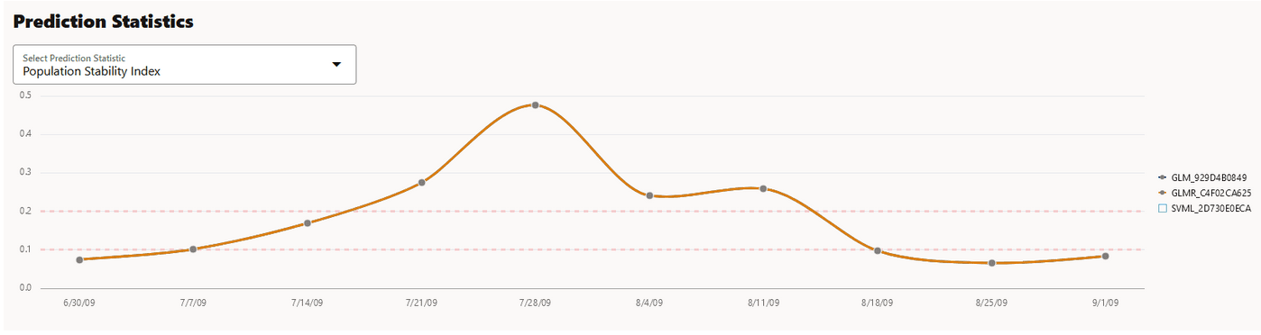
• Prediction Statistics: Scroll further down to view the Prediction Statistics section. The computed prediction statistic is plotted along the y axis, and the time period is plotted along the x axis. In this screenshot, the Population Stability Index for the Generalized Linear Model — Regression model GLMR_C4F02CA625 for 10/30/10 is displayed. Hover your cursor on other points on the line to view the computed metric.

  Figure 13: Prediction Statistics

  

  Description of the illustration model_details3.png

  Click on the drop-down list to view all the prediction statistics. The statistics of the predictions of the model vary according to the type of model.

  For Regression, the computed prediction statistics are:

  • Population Stability Index: This is a measure of how much a population has shifted over time or between two different samples of a population in a single number. The two distributions are binned into buckets, and PSI compares the percents of items in each of the buckets. PSI is computed as

    PSI = sum((Actual_% - Expected_%) x ln (Actual_% / Expected_%))

    The interpretation of PSI value is:

    • PSI < 0.1 implies no significant population change

    • 0.1 <= PSI < 0.2 implies moderate population change

    • PSI >= 0.2 implies significant population change

  • Min: This is the lowest value of the computed statistics for the analysis period.

  • Mean: This is the average value of the computed statistics for the analysis period.

  • Max: This is the highest value of the computed statistics for the analysis period.

  • Standard Deviation: This is the value that shows how much variation from the mean exists.

  For Binary Classification, the computed prediction statistics are:

  • Population Stability Index

  • Mean

  • Min

  • Max

  • Standard Deviation

  • Bin Distribution of prediction probabilities

  • Class distribution

  For Multi-class Classification, the computed prediction statistics are:

  • Population Stability Index

  • Class Distribution

2. Model Monitor Details

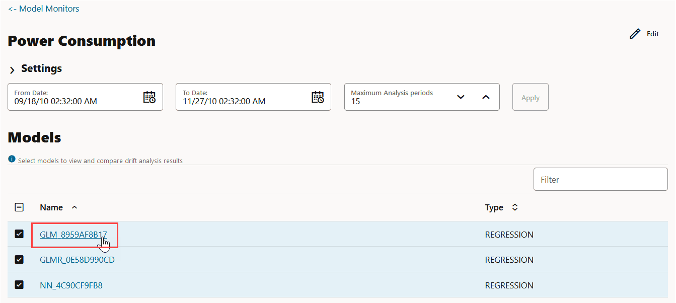
You can view the details of each feature of the model by clicking on the model name. These details include the Feature Impact chart, Prediction Distribution and the Predictive Impact versus Drift Importance chart. In this example, the model GLM_8959AF817 is selected.

Figure 14: Model selection for details

Description of the illustration view_feature_impact_mm.png

The computed results are displayed on a separate pane that slides in. You can select up to 3 analysis periods comparison. You also have the option to hide or show the baseline details. The computed details of the model features are:

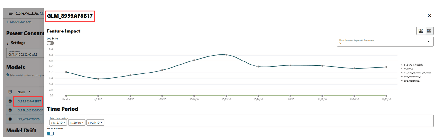
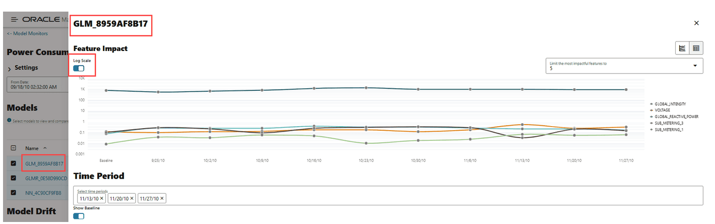
• Feature Impact: The Feature Impact chart computes the impact of each feature in the model for the specified time. The chart also the gives you the option to view the feature impact on a linear scale as well as on a logarithmic scale. Hover your mouse over the chart to view the details - Feature Name, Date, and Feature Impact.

  • Click Log Scale to view the feature impact computation on a logarithmic scale.

  • Click to view the feature impact computation in a line graph.

  • Click to view the feature impact computation in a table.

  • Click Limit the most impactful features to drop down list to select a value.

  Figure 15: Viewing Feature Impact on a liner scale

  

  Description of the illustration feature_impact_mm.png

  In this screenshot, the feature GLOBAL_INTENSITY, that is, the global minute-averaged current intensity of the household electric consumption is seen to have the maximum impact on the model GLM_8959AF817 as compared to the other features. Click on Log Scale to view feature impact computation on a logarithmic scale, as shown in the screenshot below. Click X on the top right corner of the pane to exit.

  Figure 16: Viewing Feature Impact on a Logarithmic Scale

  

  Description of the illustration feature_impact_mm_logscale.png

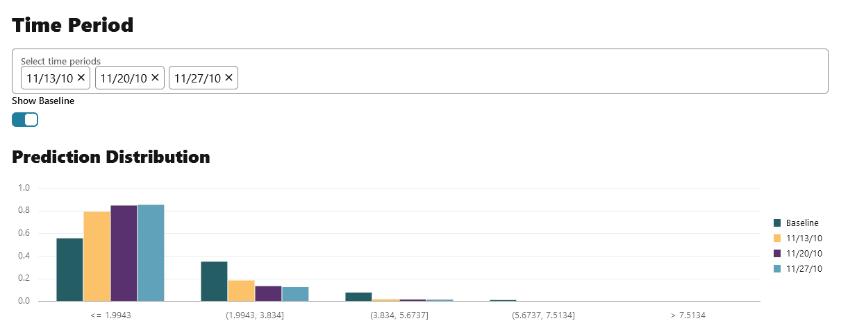
• Prediction Distribution: Scroll down to view the Prediction Distribution. Prediction Distribution is plotted for each analysis period. The Baseline data is displayed, if selected. The bins are plotted along X-axis, and the values are plotted along the Y-axis. Hover your mouse over each histogram to view the computed details. Click X on the top right corner of the pane to exit. Figure 17: Prediction Distribution

  

  Description of the illustration prediction_distribution.png

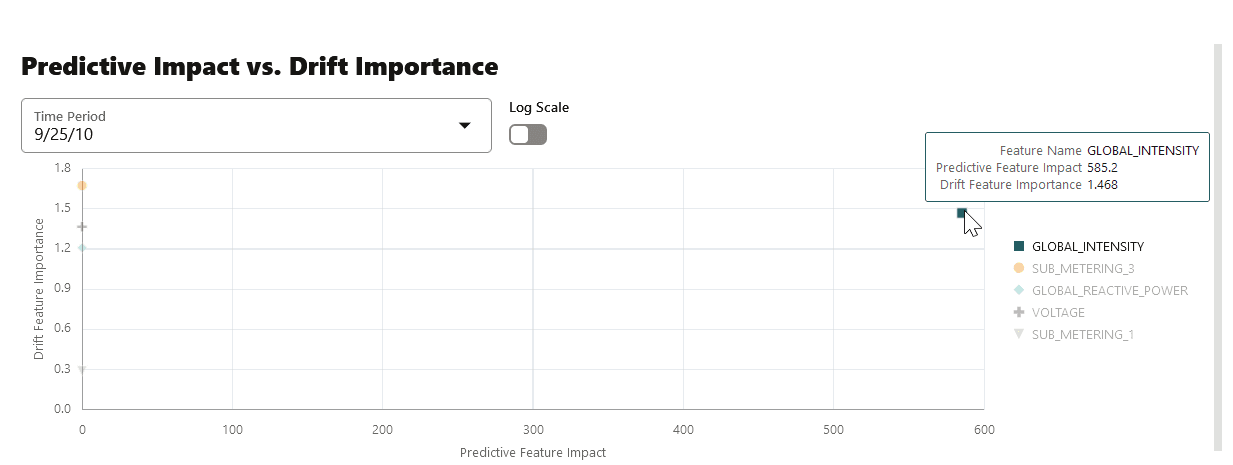
• Predictive Impact vs Drift Importance: Scroll further down the pane to view the Prediction Impact versus Drift Importance chart. This chart helps in understanding how the most impactful features drift over time. Drift Feature Importance is plotted along the Y-axis and Prediction Feature Impact is plotted along the X-axis. Click X on the top right corner of the pane to exit.

  Note: The Prediction Impact vs Drift Importance chart is computed only if you select the Monitor Data option while creating the model monitor.

  Figure 18: Predictive Feature Impact versus Drift Importance

  

  Description of the illustration prediction_drift_impact_mm.png

  In this screenshot, you can see that the feature GLOBAL_INTENSITY has the maximum impact on the selected predictive model GLM_8959AF817 as compared to the other features - SUB_METERING_3, GLOBAL_REACTIVE_POWER, VOLTAGE, and SUB-METERING_1.

View Model History

The History page displays the runtime details of the model monitors.

Select a model monitor and click History to view the runtime details. The history page displays the following information about the model monitor runtime:

Figure 19: View Model History

Description of the illustration model_history.png

• Actual Start Date: This is the date when the model monitor actually started.

• Requested Start Date: This is the date entered in the Start Date field while creating the model monitor.

• Status: The statuses are SUCCEEDED and FAILED.

• Detail: If a model monitor fails, the details are listed here.

• Duration: This is the time taken to run the model monitor.

Click Back to Monitors to go back to the Model Monitoring page.