Recommend Movies Using Association Rules

3.4 Recommend Movies Using Association Rules

A popular movie rental website is getting an update. The company wants to suggest movies to customers based on the ones they rent most often. As a data scientist, you’re tasked with helping. You apply the Apriori algorithm to identify movies that are frequently watched together, enabling the creation of smarter recommendations for users.

Topic	Link
About Associatio Rules	Association
About Model Setting	About Model Setting
Shared Settings	Shared Settings

3.4.1 Load and Examine Data

Examine the data set and its attributes. Load the data in your database.

In this use case, you will load the data set to your database. If you are using Oracle Autonomous AI Database, you will use an existing data file from the Oracle Cloud Infrastructure (OCI) Object Storage. You will create a sample table, load data into the sample table from files on the OCI Object Storage, and explore the data. If you are using the on-premises database, you will use Oracle SQL developer to import the data set and explore the data.

To understand the data, you will perform the following:

Access the data.
Examine the various attributes or columns of the data set.
Assess data quality (by exploring the data).

Load Data

To load the data in your database, run the following script.

This script connects to the database, creates a proxy object for the MOVIE_SALES_FACT table in your environment, and displays the first 10 rows for review.

%r

ore.sync(table = "MOVIE_SALES_FACT")
ore.attach()

MOVIE_SALES_FACT1 <- MOVIE_SALES_FACT
z.show(head(MOVIE_SALES_FACT1, 10))

The output appears as follows:

Examine Data

The table below shows the attributes columns in MOVIES_SALES_FACT and their descriptions:

Attribute Name	Description with Examples
ORDER_NUM	Specifies the Customer's order number, For example, 10234.
ACTUAL_PRICE	Actual price of the movie, For example, $14.99.
AGE	Age of the customer, For example, 32 years.
AGE_BAND	Age band of the customer, For example, 30-39 years.
APP	Application used for the movie, For example, Netflix.
CITY	Name of the city where the customer is located, for example, New York or Los Angeles.
CITY_ID	City ID, For example, 101.
COMMUTE_DISTANCE	Distance the customer travels from home to their primary destination. For example: 5km.
COMMUTE_DISTANCE_BAND	Range or category of commute distance for the customer, for example, 0-10 km or 10-20 km.
CONTINENT	Continent where the customer is located. For example, North America or Asia.
COUNTRY	Country where the customer resides, for example, USA or Canada.
COUNTRY_CODE	Country code for the customer’s country, for example, US or IN.
COUNTRY_ID	Unique identifier for the customer’s country, for example, 1 for the USA or 2 for Canada.
CREDIT_BALANCE	Customer’s credit balance, For example, $50.00.
CUSTOMER_ID	Customer ID, For example, C1234.
CUSTOMER_NAME	Customer name, For example, John Doe.
DAY	Date and time of the transaction in YYYY-mm-dd hh:mm:ss format, For example, 2025-10-24 14:30:00.
DAY_NAME	Day of the week, For example, Friday.
DAY_NUM_OF_WEEK	Day number of the week, For example, 5.
DEVICE	Device used by the customer, For example, iPhone 13.
DISCOUNT_PERCENT	Discount percent, For example, 10%.
DISCOUNT_TYPE	Discount type, For example, Coupon.
EDUCATION	Customer’s education, For example, Bachelor’s.
EMAIL	Customer email ID, For example, john@example.com.
FULL_TIME	Customer’s employment status, For example, Full-time.
GENDER	Gender of the customer, For example, Male.
GENRE	Movie genre, For example, Action.
HOUSEHOLD_SIZE	Household size, For example, 3 persons.
HOUSEHOLD_SIZE_BAND	Household size band, For example, 3-4 persons.
INCOME	Customer’s income, For example, $60,000 per year.
INCOME_BAND	Income band, For example, $50,000-$70,000 per year.
INSUFF_FUNDS_INCIDENTS	Number of insufficient fund incidents, For example, 1.
JOB_TYPE	Customer’s job, For example, Engineer.
LATE_MORT_RENT_PMTS	Customer had any late mortgage or rent payments, For example, Yes.
LIST_PRICE	List price of the movie, For example, $19.99.
MARITAL_STATUS	Marital status of the customer, For example, Married.
MONTH	Month in MON-YYYY format, where MON is the three-letter month abbreviation (Jan–Dec). Example: Oct-2025.
MONTH_NAME	Month name, For example, October.
MONTH_NUM_OF_YEAR	Month of purchase number of the year, For example, 10.
MORTGAGE_AMT	Mortgage amount, For example, $250,000.
MOVIE_ID	Movie ID, For example, M101.
NUM_CARS	Number of cars the customer owns, For example, 2 cars.
NUM_MORTGAGES	Number of mortgages, For example, 1.
OS	OS information, For example, iOS.
PAYMENT_METHOD	Payment method, For example, Credit Card.
PET	Specifies if the customer owns a pet, For example, Yes.
POSTAL_CODE	Postal code, For example, 10001.
PROMOTION_RESPONSE	Specifies the response to a promotional offer, For example, Accepted.
QUANTITY_SOLD	Quantity sold, For example, 1 copy.
QUARTER_NAME	Quarter name in Qn-YYYY format, For example, Q4-2025.
QUARTER_NUM_OF_YEAR	Quarter number of the year, For example, 4.
RENT_OWN	Specifies if the customer lives in a rented or owned place, For example, Own.
SEARCH_GENRE	Genre of movies searched, For example, Thriller.
SEGMENT_DESCRIPTION	Describes the population segment, For example, High-income urban.
SEGMENT_NAME	Population segment name, For example, Urban Premium.
SKU	SKU ID, For example, SKU1234.
STATE_PROVINCE	Province or state, For example, New York.
STATE_PROVINCE_ID	Province ID, For example, 33.
STREET_ADDRESS	Customer’s street address, For example, 123 Main Street.
TITLE	Movie title, For example, Air Force One.
USERNAME	Username provided by the customer, For example, johndoe123.
WORK_EXPERIENCE	Work experience of the customer, For example, 8 years.
WORK_EXPERIENCE_BAND	Work experience band, For example, 5-10 years.
YEAR	Year of transaction, For example, 2025.
YEARS_CURRENT_EMPLOYER	Years with current employer, For example, 5 years.
YEARS_CURRENT_EMPLOYER_BAND	Customer’s employment band with current employer, For example, 3-5 years.
YEARS_RESIDENCE	Number of years at current residence, For example, 7 years.
YEARS_RESIDENCE_BAND	Residence band, For example, 5-10 years.

Parent topic: Recommend Movies Using Association Rules

3.4.2 Explore Data

Once the data is loaded into the table, explore the data to understand and assess the quality of the data. At this stage assess the data to identify data types and noise in the data. Look for missing values and numeric outlier values.

Follow the steps below to understand the data:

Check the dimensions (rows and columns) of the MOVIE_SALES_FACT1 table.
To display number of rows and columns in the MOVIE_SALES_FACT1 table, run the following script:
```
%r

dim(MOVIE_SALES_FACT1)
```
```
1957811240.70
```
Find movie sales information for a specific customer

The script filters the MOVIE_SALES_FACT1 dataset to retrieve records where CUSTOMER_ID = 1000050, and selects the columns ORDER_NUM, MONTH, CUSTOMER_ID, MOVIE_ID, TITLE, GENRE, ACTUAL_PRICE, and QUANTITY_SOLD. It then displays the first few rows of the filtered result using z.show(head(MOVIE_SALES_SELECT)).
```
%r

MOVIE_SALES_SELECT <- MOVIE_SALES_FACT1 %>%
  filter(CUSTOMER_ID == 1000050) %>%
  select(ORDER_NUM, MONTH, CUSTOMER_ID, MOVIE_ID, TITLE, GENRE, ACTUAL_PRICE, QUANTITY_SOLD)

z.show(head(MOVIE_SALES_SELECT))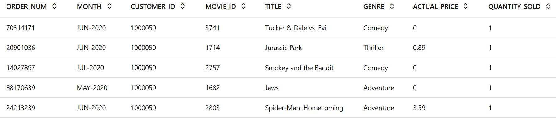
```
Run the following script to display the data types of the attributes.

This script retrieves and displays the structural description (desc) of the MOVIE_SALES_FACT1 object.
```
%r

MOVIE_SALES_FACT1@desc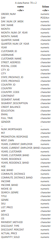
```
This output displays the data types of the attributes in the dataset.
The dataset contains millions of records. To narrow down the results, create a view named MOVIES that filters the data based on specific criteria.

This script creates or updates a view called MOVIES that contains unique combinations of CUSTOMER_ID, MOVIE_ID, and TITLE for customers whose CUSTOMER_ID is between 1000050 and 1010000, and movies sold in FEB-2018. It further applies a filtering condition to keep approximately 5% of the rows per customer, based on a mathematical condition involving CUSTOMER_ID and MOVIE_ID. The resulting view is pulled into MOVIES_df, and the first few rows of the dataset are displayed using z.show(MOVIES_df).
```
%r

MOVIES <- MOVIE_SALES_FACT1 %>%
  filter(MONTH == "FEB-2018") %>%
  filter(CUSTOMER_ID >= 1000050 & CUSTOMER_ID <= 1010000) %>%
  select(CUSTOMER_ID, MOVIE_ID, TITLE) %>%
  distinct() %>%
  filter((CUSTOMER_ID * 31 + MOVIE_ID * 17) %% 20 == 0)  # Keep ~5% of rows per customer
  MOVIES_df <- ore.pull(MOVIES)
  z.show(MOVIES_df)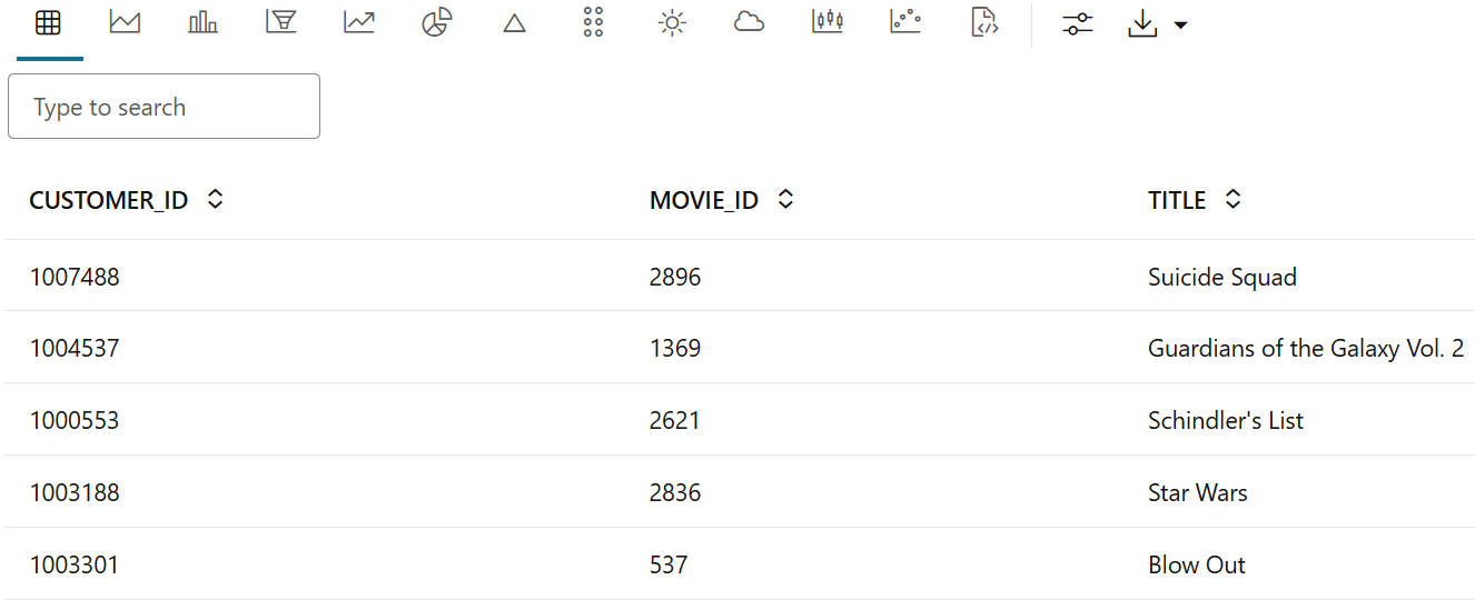
```
The output appears as follows:
Identify popular movies watched by customers who watched Titanic

The script identifies customers who watched Titanic, then finds other movies watched by those customers. It counts the number of customers who watched each movie, filters out movies watched by fewer than 100 customers, and displays the top 20 most popular movies.
```
%r

titanic_ids <- ore.pull(
  MOVIE_TRANSACTIONS %>%
    filter(TITLE == "Titanic") %>%
    select(CUSTOMER_ID)
)$CUSTOMER_ID

cat("Titanic customers in dataset:", length(titanic_ids), "\n")

popular_movies_df <- ore.pull(
  MOVIE_TRANSACTIONS %>%
    filter(CUSTOMER_ID %in% titanic_ids &
           TITLE != "Titanic") %>%
    group_by(TITLE) %>%
    summarise(CUSTOMER_COUNT = length(TITLE)) %>%
    arrange(desc(CUSTOMER_COUNT))
)

z.show(head(popular_movies_df, 20))
```
The output appears as follows:

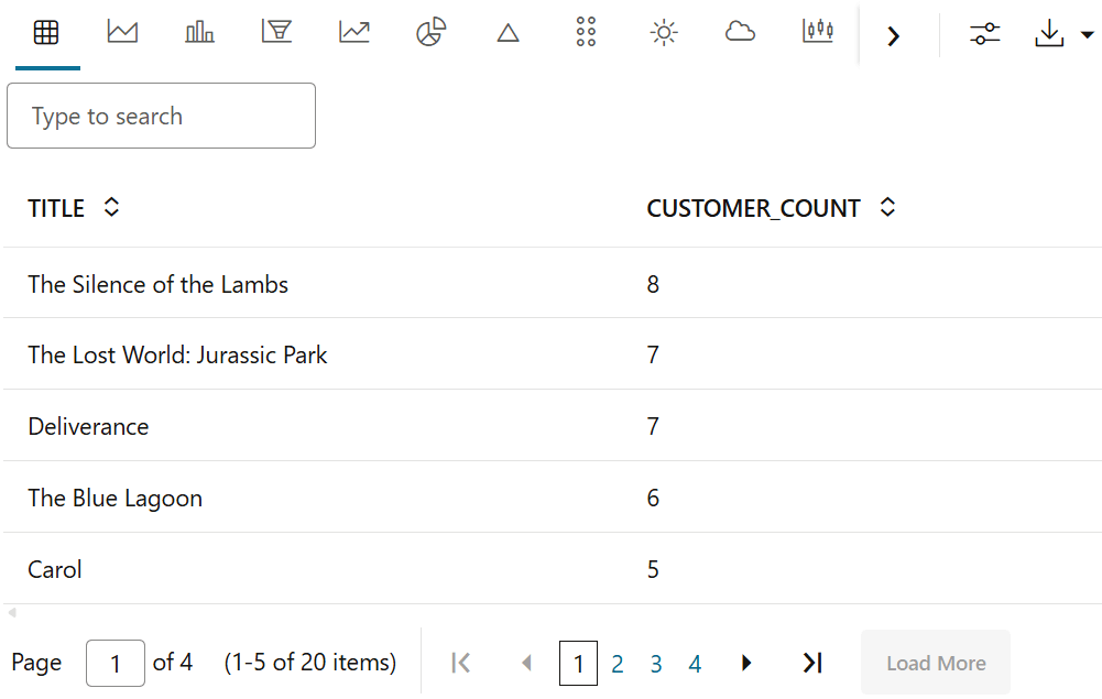
These results represent the most popular movies among customers who had previously purchased or viewed Titanic.
To check if there are any missing (NULL) values, run the following script:
```
%r

NULL_COUNT <- MOVIES %>%
  filter(is.na(CUSTOMER_ID) | is.na(TITLE)) %>%
  nrow()

z.show(data.frame(NULL_COUNT = NULL_COUNT))
```
```
NULL_COUNT 
0
```
The result NULL_COUNT = 0 indicates that there are no missing values (NA) in the critical columns (CUSTOMER_ID and TITLE) of the MOVIES dataset.

This means that your dataset is clean in terms of these two columns, and no further data cleaning steps are needed for missing values in these specific fields.
Extract the relevant data

To extract the relevant data from the cleaned dataset, selecting only the CUSTOMER_ID and TITLE columns, run the following script. This step is important for preparing the data, where customer movie purchases are treated as transactions and movie titles as items.
```
%r

MOVIE_TRANSACTIONS <- MOVIES %>%
  select(CUSTOMER_ID, TITLE) %>%
  distinct()

z.show(head(ore.pull(MOVIE_TRANSACTIONS), 10))
```
The output appears as follows:

Parent topic: Recommend Movies Using Association Rules

3.4.3 Build Model

To build your Association Rules model, use the ore.odmAssocRules function to derive rules from the movie-stream dataset. This is an unsupervised technique—the algorithm identifies naturally occurring co-occurrence patterns in the data. Because of this, you do not split the data into training and test sets, and you do not evaluate accuracy as you would with supervised models.

In this use case, the data captures sets of movies viewed together. The algorithm scans these sets to find frequently co-watched titles and relationships among selections.

For example, the model discovers patterns like:

Customers who watched Movie A and Movie B often also watch Movie C.
Movie X and Movie Y frequently appear together in many customers’ viewing histories.

These patterns form association rules, such as: {Movie A, Movie B} → {Movie C}

For each rule, the algorithm reports objective measures, including:

Support: how frequently the itemset appears.
Confidence: how often the right-hand side appears when the left-hand side is present.
Lift: how much more likely the right-hand side is given the left-hand side compared to chance.

Not all rules are equally strong. Recommendations should be driven by rules that meet your selected thresholds for support, confidence, and lift. The value of the model is that it provides data-driven suggestions by identifying natural relationships between movies:

If a user’s viewing history matches a rule’s left-hand side, recommend items on the right-hand side from rules that satisfy your minimum support/confidence/lift thresholds.
The rules enable personalized recommendations based on observed viewing patterns.
Unlike content-based filtering, this method does not rely on movie metadata (genre, actors, etc.); recommendations are derived from observed co-occurrences.

Algorithm Selection

The Apriori algorithm discovers frequent itemsets and generates association rules from transactional data. In this notebook, the algorithm identifies combinations of movie titles that are frequently watched together by customers.

How It Works

The algorithm operates in two stages. First, it identifies frequent itemsets — groups of movies that appear together across customer watch histories in MOVIE_TRANSACTIONS, where each customer is a transaction and each movie title is an item. Second, it generates association rules describing the likelihood of a customer watching one movie based on their history of watching another. For example: "Customers who watched Venom are also likely to watch Captain America: The Winter Soldier."

Key Metrics

Support: the proportion of all customers in MOVIE_TRANSACTIONS who watched both movies together. A min.support = 0.03 means a movie pair must appear in at least 3% of all customer baskets to be considered.
Confidence: the probability that a customer who watched Movie A also watched Movie B. A min.confidence = 0.3 means at least 30% of customers who watched the antecedent also watched the consequent.
Lift: measures how much more likely two movies are watched together compared to by chance. A lift > 2.0 filter is applied throughout this notebook to surface only genuinely non-trivial associations.
Reverse Confidence: the probability in the opposite direction: given a customer watched the recommended movie (RHS), how likely are they to have also watched the trigger movie (LHS). Calculated as support × lift / confidence.

Building the Model with Apriori

To build the model, you will use the ore.odmAssocRules function, which uses the in-database Apriori algorithm to find frequent item sets and generate association rules. Set the hyperparameters for the model, such as minimum support, minimum confidence, and the maximum rule length, as shown in the following script:

ar.mod1 <- ore.odmAssocRules(
  ~.,
  data            = MOVIE_TRANSACTIONS,
  case.id.column  = "CUSTOMER_ID",
  item.id.column  = "TITLE",
  min.support     = 0.03,   # 3% of 115 customers = ~3-4 customers per rule
  min.confidence  = 0.3,    # 30% confidence
  max.rule.length = 2
)

Explanation:

ore.odmAssocRules: This function builds the Association Rules model using the Apriori algorithm.
case.id.column: Specifies the column representing the unique transaction identifier (in this case, CUSTOMER_ID).
item.id.column: Specifies the column representing the items (movies in this case) in the transactions (TITLE).
min.support: Minimum support threshold for the itemsets to be considered frequent. It is set at 0.03 (3%), meaning an itemset must appear in at least 3-4 customers' transactions out of 115 total transactions to be considered frequent.
min.confidence: Minimum confidence for the association rules. In this case, a rule must have at least 30% confidence to be considered valid. This means that, for example, 30% of the time when one item (movie) is purchased, the rule predicts the purchase of another item (movie).
max.rule.length: Specifies the maximum number of items allowed in the association rules. In this case, rules can involve up to 2 items, which means the rules will capture relationships between pairs of items (both an antecedent and a consequent). Limiting the rule length helps manage the complexity of the model, keeping it focused on simpler, interpretable patterns. Choosing higher values for rule length could increase computational demands, impacting performance and memory usage.

Parent topic: Recommend Movies Using Association Rules

3.4.4 Evaluate

After building your association rules model, the next step is to evaluate the quality of the generated rules. Evaluation helps determine how well the model identifies meaningful relationships between items in the dataset.

Since association rule learning is an unsupervised technique, traditional metrics like accuracy are not available. Instead, the focus is on understanding the generated rules and the statistical measures that indicate their strength and relevance.

Key Metrics for Evaluating Association Rules

The evaluation of association rules primarily involves three key metrics:

Support: Represents how frequently the items in the rule (the antecedent and consequent) appear together in the dataset. In this context, support indicates the proportion of all user sessions where both movies (For example, "The Dark Knight" and "Inception") are watched together. For example, if 25% of all user sessions include both movies, the support for the rule is 25%. This metric helps determine the relevance of the association, with higher support values indicating more commonly occurring patterns.
Confidence: Measures the likelihood that the consequent (right-hand side) occurs when the antecedent (left-hand side) is present in a transaction. In this case, confidence assesses how reliably the rule predicts that a user who watches the antecedent movie (For example, "The Dark Knight") will also watch the consequent movie (For example, "Inception"). For example, if 80% of users who watch "The Dark Knight" also watch "Inception," the confidence of this rule would be 80%. This gives a measure of how dependable the association is in predicting user behavior.
Lift: Measures the strength of an association between items by comparing the observed co-occurrence with the expected co-occurrence if the items were independent. In this case, a lift value greater than 1 indicates that the movies are more likely to be watched together than by random chance, suggesting a strong association. A lift value below 1 implies the association is weak or not meaningful.

These metrics help rank the rules and identify those most valuable for business or analysis purposes.

Evaluating the Model Output

Once the model is built and the association rules are extracted, the quality of the rules can be evaluated by examining these metrics. The goal is to identify rules that reveal meaningful patterns, such as frequently bought items, and have high support, confidence, and lift.

The evaluation process involves inspecting the rules. After building the model using the Apriori algorithm, review the support, confidence, and lift of each rule. This evaluation helps assess the relevance of the rules for potential applications, such as recommendations. You can extract and manipulate the generated rules using functions like rules(ar.mod1) and view the summary of metrics for each rule.

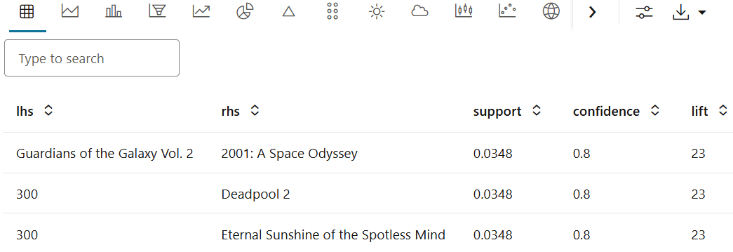
To extract the association rules from the ar.mod1 model and inspect the top 3 rules to evaluate their support, confidence, and lift values, use the following script:
```
%r

# Extract association rules from the model and inspect top 3 by lift
ar.rules.local <- ore.pull(rules(ar.mod1))

rules.df <- data.frame(
  lhs        = gsub("[{}]", "", labels(lhs(ar.rules.local))),
  rhs        = gsub("[{}]", "", labels(rhs(ar.rules.local))),
  support    = round(ar.rules.local@quality$support,    4),
  confidence = round(ar.rules.local@quality$confidence, 4),
  lift       = round(ar.rules.local@quality$lift,       4)
) %>%
  filter(confidence < 1.0 & lift > 2.0) %>%
  arrange(desc(lift), desc(confidence))

z.show(head(rules.df[, c("lhs", "rhs", "support", "confidence", "lift")], 3))
```
The output appears as follows:

The output shows:

Three association rules generated from the data, each consisting of the left-hand side (lhs) (antecedent or trigger of the rule), right-hand side (rhs) (consequent or outcome of the rule), and three important metrics: support (frequency of rule occurrence), confidence (probability that the consequent appears when the antecedent is present), and lift (degree of association between the items).
- Support = 0.0348 for all top rules indicates that approximately 3.5% of all customers in the dataset watched both the LHS and RHS movies together.
- Confidence = 0.8 for all top rules means that 80% of customers who watched the trigger movie (LHS) also watched the recommended movie (RHS).
- Lift = 23 for all top rules indicates that customers who watched the LHS movie are 23 times more likely than average to have also watched the RHS movie.
The output indicates that the rules are highly reliable in predicting the co-occurrence of items based on the observed data.

To see top 10 association rules, run the following query:

This script extracts the association rules from the ar.mod1 model, sorts them based on confidence and support, and then displays the top 10 highest-ranking rules based on those metrics.

%r

ar.rules <- ore.pull(rules(ar.mod1))

df <- data.frame(
  lhs        = gsub("[{}]", "", labels(lhs(ar.rules))),
  rhs        = gsub("[{}]", "", labels(rhs(ar.rules))),
  support    = round(ar.rules@quality$support,    4),
  confidence = round(ar.rules@quality$confidence, 4),
  lift       = round(ar.rules@quality$lift,       4)
)

# Filter out trivial and perfect rules, sort by confidence then support
df <- df[df$confidence < 1.0 & df$lift > 2.0, ]
df <- df[order(-df$confidence, -df$support), ]

z.show(head(df[, c("lhs", "rhs", "support", "confidence", "lift")], 10))

The output appears as follows:

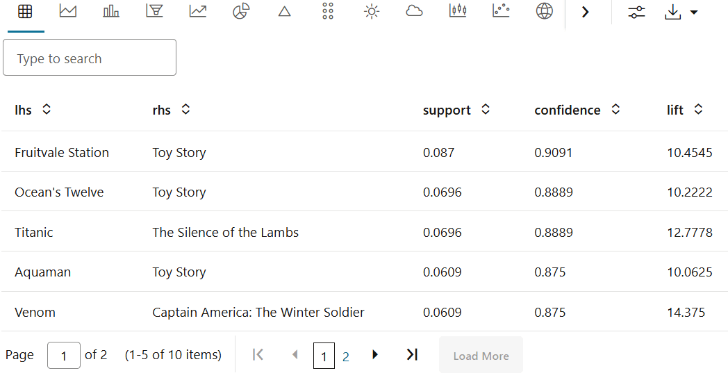
The diagram displays the top 10 highest-ranking rules based on those metrics.

The output displays the top 10 association rules sorted byconfidence and support.

To see which consequent items appear most frequently or are in the most rules, run the following script:

The script extracts the right-hand side (consequents) of association rules, cleans up the consequents (the process of removing unwanted characters or formatting from the extracted consequents), counts the frequency of each unique consequent.
```
%r

# Pull rules and build clean data frame
ar.rules.local <- ore.pull(rules(ar.mod1))

df <- data.frame(
  rhs        = gsub("[{}]", "", labels(rhs(ar.rules.local))),
  confidence = ar.rules.local@quality$confidence,
  lift       = ar.rules.local@quality$lift
)

# Filter trivial and perfect rules before aggregating
# Same filter as working code above — confidence < 1.0 and lift > 2.0
consequents_df <- df %>%
  filter(confidence < 1.0 & lift > 2.0) %>%
  group_by(rhs) %>%
  summarise(CNT = length(rhs)) %>%
  arrange(desc(CNT))

names(consequents_df) <- c("CONSEQUENT", "CNT")

z.show(consequents_df)
```
The output appears as follows:

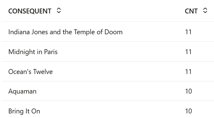
This output shows a table that contains two columns:
- consequents: These are the items or item sets that appear on the right-hand side (RHS) of the association rules.
- CNT: This is the frequency count of how often each consequent appears across the association rules.

To see which antecedent items occur most frequently or which antecedent items are included in most rules, run the following script:

This script extracts, cleans, and counts the most frequent antecedents (LHS) of the association rules.

%r

ar.rules.local <- ore.pull(rules(ar.mod1))
rules.df <- data.frame(
  lhs        = gsub("[{}]", "", labels(lhs(ar.rules.local))),
  confidence = ar.rules.local@quality$confidence,
  lift       = ar.rules.local@quality$lift
)

# Filter trivial and perfect rules before aggregating — consistent with working code
antecedent.freq <- rules.df %>%
  filter(confidence < 1.0 & lift > 2.0) %>%
  group_by(lhs) %>%
  summarise(RULE_COUNT = length(lhs)) %>%
  arrange(desc(RULE_COUNT))

# cat("Distinct antecedents:", nrow(antecedent.freq), "\n\n")
z.show(head(antecedent.freq, 20))

The output appears as follows:

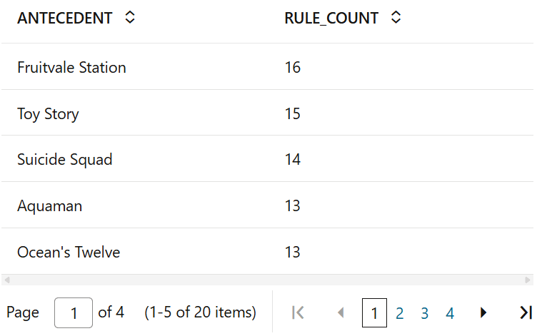
The diagram displays the antecedent items that occur most frequently or which antecedent items are included in most rules.

The output generates the table that lists each antecedent (item) and its frequency count, sorted by how often each antecedent appears across all the rules.

To check how many rules show up in each band of support, run the following script:

This script divides the support values of the association rules into bins (ranges) using specified breakpoints (bin_breaks). It assigns a label to each bin (e.g., (0.03,0.06], (0.06,0.09], etc.) and then counts how many rules fall into each bin using table(). Finally, it displays the distribution of these counts in a bar plot, showing how the support values of the rules are distributed across different support ranges.

%r

ar.rules.local <- ore.pull(rules(ar.mod1))
rules.df <- data.frame(
  lhs        = gsub("[{}]", "", labels(lhs(ar.rules.local))),
  rhs        = gsub("[{}]", "", labels(rhs(ar.rules.local))),
  support    = round(ar.rules.local@quality$support,    4),
  confidence = round(ar.rules.local@quality$confidence, 4),
  lift       = round(ar.rules.local@quality$lift,       4)
)

# Apply consistent filter
rules.df <- rules.df[rules.df$confidence < 1.0 & rules.df$lift > 2.0, ]

# Use narrow bin breaks matching actual support range (0.03 to 0.12)
bin_breaks <- seq(0, 0.15, by = 0.03)
bin_labels <- paste0("(", head(round(bin_breaks, 3), -1), ",",
                          tail(round(bin_breaks, 3), -1), "]")

rules.df$supp_bin <- cut(rules.df$support,
                         breaks = bin_breaks,
                         include.lowest = TRUE,
                         labels = bin_labels)

# Count rules per bin
supp_bins_df <- rules.df %>%
  group_by(supp_bin) %>%
  summarise(RULE_COUNT = length(lhs)) %>%
  arrange(supp_bin)

# Display — choose barplot, set RULE_COUNT as Series, supp_bin as Group By
# Change aggregation from Average to Sum in chart settings
z.show(supp_bins_df)

The output appears as follows:

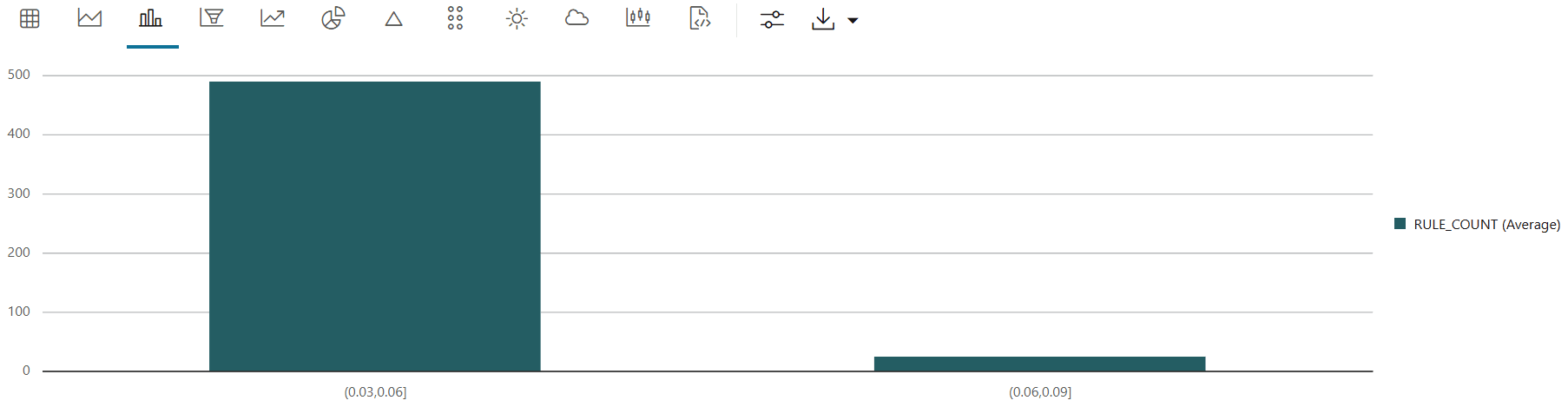
The diagram displays the many rules that show up in each band of support.

The output, a bar plot, visually represents how the support values of association rules are distributed across different support ranges (bins).

The plot helps identify:

The frequency of rules within each support range.
The concentration of rules in lower or higher support ranges.
The general popularity or strength of the association rules based on their support.

To check how many rules show up in each band of confidence, run the following query:

This code bins the confidence values of association rules into predefined intervals and then creates a bar plot to visualize the distribution of these binned values.

%r

ar.rules.local <- ore.pull(rules(ar.mod1))
rules.df <- data.frame(
  lhs        = gsub("[{}]", "", labels(lhs(ar.rules.local))),
  rhs        = gsub("[{}]", "", labels(rhs(ar.rules.local))),
  support    = round(ar.rules.local@quality$support,    4),
  confidence = round(ar.rules.local@quality$confidence, 4),
  lift       = round(ar.rules.local@quality$lift,       4)
)

# Apply consistent filter
rules.df <- rules.df[rules.df$confidence < 1.0 & rules.df$lift > 2.0, ]

# Bin breaks matching actual confidence range (0.3 to 1.0)
bin_breaks <- seq(0.3, 1.0, by = 0.1)
bin_labels <- paste0("(", head(round(bin_breaks, 2), -1), ",",
                          tail(round(bin_breaks, 2), -1), "]")

rules.df$conf_bin <- cut(rules.df$confidence,
                         breaks = bin_breaks,
                         include.lowest = TRUE,
                         labels = bin_labels)

# Count rules per confidence bin
conf_bins_df <- rules.df %>%
  group_by(conf_bin) %>%
  summarise(RULE_COUNT = length(lhs)) %>%
  arrange(conf_bin)

# Display — choose barplot, set RULE_COUNT as Series, conf_bin as Group By
z.show(conf_bins_df)

The output appears as follows:

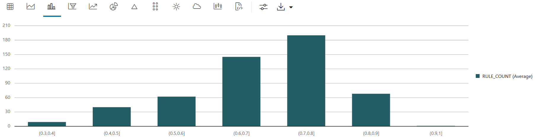
The diagram displays the many rules that show up in each band of confidence.

The output bar plot visually represents how the confidence values of the association rules are distributed across different confidence intervals, allowing you to easily see the frequency of rules in each bin.

To get the top 5 movie recommendations for a customer based on their selected movies using an association rules model, run the following script:

This code defines a function get_top5_customer_recommendations that recommends movies to a customer based on association rules from a model. It filters the rules to find those that are relevant to the customer's selected movies and calculates various quality metrics (e.g., support, confidence, lift, reverse confidence) for the recommendations. The top 5 recommendations are ranked by confidence and support, excluding already selected movies.
```
%r

get_top5_customer_recommendations <- function(customer_movies, ar_model) {

  ar.rules.local <- ore.pull(rules(ar_model))

  rules.df <- data.frame(
    lhs        = gsub("[{}]", "", labels(lhs(ar.rules.local))),
    rhs        = gsub("[{}]", "", labels(rhs(ar.rules.local))),
    support    = round(ar.rules.local@quality$support,    4),
    confidence = round(ar.rules.local@quality$confidence, 4),
    lift       = round(ar.rules.local@quality$lift,       4),
    # FIX: Add reverse_confidence at source so it is available for aggregation
    reverse_confidence = round(ar.rules.local@quality$support *
                               ar.rules.local@quality$lift /
                               ar.rules.local@quality$confidence, 4),
    stringsAsFactors = FALSE
  )

  rules.df <- rules.df[rules.df$confidence < 1.0 & rules.df$lift > 2.0, ]
  rules.df <- rules.df[rules.df$lhs %in% customer_movies, ]

  if (nrow(rules.df) == 0) {
    message("No recommendations found for: ", paste(customer_movies, collapse = ", "))
    return(data.frame())
  }

  rules.df <- rules.df[!(rules.df$rhs %in% customer_movies), ]

  if (nrow(rules.df) == 0) {
    message("No recommendations left after removing already selected movies.")
    return(data.frame())
  }

  result_final <- rules.df %>%
    group_by(rhs) %>%
    summarise(
      COUNT              = length(rhs),
      SUPPORT            = round(mean(support),            3),
      CONFIDENCE         = round(mean(confidence),         3),
      LIFT               = round(mean(lift),               3),
      # FIX: Include reverse_confidence in aggregation
      REVERSE_CONFIDENCE = round(mean(reverse_confidence), 3)
    ) %>%
    arrange(desc(CONFIDENCE), desc(SUPPORT)) %>%
    slice_head(n = 5)

  names(result_final)[1] <- "RECOMMENDATION"
  result_final$RANK <- seq_len(nrow(result_final))

  # FIX: Include REVERSE_CONFIDENCE in final column selection
  result_final <- result_final[, c("RANK", "RECOMMENDATION", "COUNT",
                                   "SUPPORT", "CONFIDENCE", "LIFT",
                                   "REVERSE_CONFIDENCE")]
  return(result_final)
}

customer_selection <- c("Avatar")
top5_recommendations <- get_top5_customer_recommendations(customer_selection, ar.mod1)
z.show(top5_recommendations)
```
The output appears as follows:

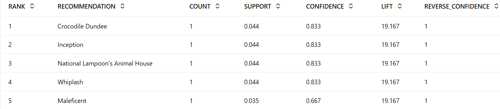
The output of the code displays the top 5 movie recommendations for a customer based on their selected movies, along with key metrics for each recommendation. The columns in the output include:
- RANK: The rank of each recommendation based on its confidence and support.
- RECOMMENDATION: The movie recommended to the customer. This represents the right-hand side (RHS) of the association rule generated from the selected movie(s).
- COUNT: The number of filtered association rules that produced this specific recommendation. A value of 1 indicates that exactly one rule matched for that recommendation.
- SUPPORT: The support of the rule, representing the proportion of transactions in which both the antecedent and consequent items (the selected movie and the recommended movie) appear together.
- CONFIDENCE: Represents the probability that a customer will watch the recommended movie given that they have already watched the selected movie.
- LIFT: A measure of how much more likely the recommended movie is watched when the selected movie is watched, compared to independent viewing. A lift of 19.167 reflects a strong and meaningful association between the movie pair.
- REVERSE_CONFIDENCE: The ratio of the rule’s support to the overall coverage of the recommended movie (i.e., the probability that the selected movie is watched given that the recommended movie is watched). A value of 1.0 indicates that every customer who watched the recommended movie also watched the selected movie.

To conclude, you have successfully examined association rules and provided top movie recommendations to customers based on their frequently purchased and/or rented movies.

Parent topic: Recommend Movies Using Association Rules