Regression Use Case Scenario

A real estate agent approaches you, a data scientist, to provide assistance in evaluating house prices in Boston. The agent requires this information on a daily basis to provide targeted services to clients. Using the Generalized Linear Model algorithm for Regression, you estimate the median value of owner-occupied homes in the Boston area.

Topic	Link
OML4SQL GitHub Example	Regression - GLM
`CREATE_MODEL2` Procedure	CREATE_MODEL2 Procedure
Generic Model Settings	DBMS_DATA_MINING - Model Settings
Generalized Linear Model Settings	DBMS_DATA_MINING - Algorithm Settings: Generalized Linear Models
Data Dictionary Settings	Oracle Machine Learning Data Dictionary Views
Generalized Linear Model - Model Detail Views	Model Detail Views for Generalized Linear Model
About Regression	About Regression
About Generalized Linear Model (GLM)	About Generalized Linear Models

Load Data

Examine the data set and its attributes. Load the data in your database.

In this use case, you will modify the data set to add a column and upload the data set to your database. If you are using the Oracle Autonomous Database, you will upload files to the Oracle Cloud Infrastructure (OCI) Object Storage, create a sample table, load data into the sample table from files on the OCI Object Storage, and explore the data. If you are using the on-premises database, you will use Oracle SQL developer to import the data set and explore the data.

Examine Data

There are 13 attributes in the data set. This is a customized data set that excludes one attribute from the original data set. The following table displays information about the data attributes:

Attribute Name	Information
CRIM	Per capita crime rate by town
ZN	The proportion of residential land zoned for lots over 25,000 sq.ft.
INDUS	The proportion of non-retail business acres per town
CHAS	Charles River dummy variable (= 1 if tract bounds river; 0 otherwise)
NOX	Nitric oxides concentration (parts per 10 million)
RM	The average number of rooms per dwelling
AGE	The proportion of owner-occupied units built before 1940
DIS	Weighted distances to five Boston employment centers
RAD	Index of accessibility to radial highways
TAX	Full-value property-tax rate per $10,000
PTRATIO	The pupil-teacher ratio by town
LSTAT	% lower status of the population
MEDV	The median value of owner-occupied homes in $1000’s

Related Topics

How ADP Transforms the Data

Add a Column

In this data set, no row identifier uniquely identifies each record in the data set. Add a new case_id column. The case_id assists with reproducible results, joining scores for individual customers with other data in, example, scoring data table.

Add a column called House ID (HID). The HID value is added as a primary key to the table so that identifying and retrieving each record is simple. Each record in the database is called a case and each case is identified by a case_id. Here, HID is the case_id.

To add the HID column:

Open the .csv file in a spreadsheet.
Delete the first row with 506 and 13. Now, the row with the column names becomes the first row.
To the left of the data set, add a column.
Enter HID as the column name.
In the HID column enter 1 as the first value identifying the first row.
You will see a + icon in the spreadsheet cell. Drag the + icon right to the bottom till the end of the records.
Right-click and select Fill Series.
To remove the column "B" from the data set, select the entire column with the title B by right clicking on the top of the column, and then select Delete.

Import Data

There are various methods to import data into the database. Two methods are explained here. One using SQL Developer (for on-premises) and the other using Object Storage (for Cloud).

Import Data into the Database (On premises)

To access the data set, import the modified data set into the database using SQL Developer.

The following steps help you to import the data set into an on premises database.

(Optional) Enter task prerequisites here.

Launch SQL Developer on your system.
Import the modified .csv file. See Tables.
Set House ID (HID) as a primary key. This column identifies each record and helps in retrieving information about a specific record. The HID column helps when you join tables or views. See Primary Key Constraint.

You are now ready to query the table in SQL Developer.

Import Data to the Cloud

If you are using a cloud account, one of the methods of importing the data is through Object Storage. Upload the data set to an Object Storage. The Object Storage URI will be used in another procedure.

You can load data into your Oracle Autonomous Database (Autonomous Data Warehouse [ADW] or Autonomous Transaction Processing [ATP]) using Oracle Database tools, and Oracle and 3rd party data integration tools. You can load data:

from local files in your client computer, or
from files stored in a cloud-based object store

Follow the steps to upload your data file to the Object Storage bucket.

Login to your cloud account.
Click the left-side hamburger menu and select Storage from the menu.
Select Buckets from the Object Storage & Archive Storage option.
Select the compartment in which you want to upload the data.
Click Create Bucket.
Enter a name for your bucket. For example, Bucket1. Leave the rest of the fields as default.
Click Create.
Click on the bucket that you created. Scroll down and click Upload under Objects.
Leave the Object Name Prefix field black. Click select files to navigate to the data file that you want to upload or drag and drop the data file. In this use case, select the modified .csv file.
Click Upload. The data file appears under Objects.
Click the ellipses on the right side of the data file to view the menu. Click View Object Details.
Copy the URL PATH (URI) to a text file. This URI is used in the DBMS_CLOUD.COPY_DATA procedure.

This procedure creates an object storage containing the data file in your cloud account.

Create Auth Token

The Auth Token is required in the DBMS_CLOUD.CREATE_CREDENTIAL procedure. You can generate the Auth Token in your cloud account.

Login into your ADW Cloud account.
Hover your mouse cursor over the human figure icon at the top right of the console and click User Settings from the drop-down menu.
Click Auth Tokens under Resources on the left of the console.
Click Generate Token. A pop-up dialog appears.
Enter a description (optional).
Click Generate Token.
Copy the generated token to a text file. The token does not appear again.
Click Close.

Create Object Storage Credential

The object storage credential is used in the DBMS_CLOUD.COPY_DATA procedure.

Login to the OML Notebooks page and create a notebook. See Create a Notebook.
Open the notebook that you just created.
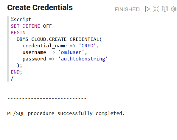
Enter the following query to create an object storage credentials:
```
%script
begin
  DBMS_CLOUD.create_credential (
    credential_name => 'CRED',
    username => '<your cloud account username>',
    password => '<your Auth Token>'
  );
end;
/
```
```
---------------------------  PL/SQL procedure successfully completed.
    ---------------------------
```
Examine the query:
- credential_name: The name of the credential to be stored. Provide any name. Here, CRED is the name given.
- username: This is your cloud account username.
- password: Enter your Auth Token password that you copied after generating the Auth Token.
Click the play icon to run the query in your notebook. Your credentials are stored in the ADW user schema.
In another para, run the following query to check the user credentials:
```
SELECT* FROM USER_CREDENTIALS;
```

Create a Table

Create a table called BOSTON_HOUSING. This table is used in DBMS_CLOUD.COPY_DATA procedure to access the data set.

Enter the following code in a new pare of the notebook that you created and run the notebook.

%sql
CREATE table boston_housing
(
 HID NUMBER NOT NULL,
 CRIM NUMBER,
 ZN NUMBER,
 INDUS NUMBER,
 CHAS VARCHAR2(32),
 NOX NUMBER,
 RM NUMBER,
 AGE NUMBER,
 DIS NUMBER,
 RAD NUMBER,
 TAX NUMBER,
 PTRATIO NUMBER,
 LSTAT NUMBER,
 MEDV NUMBER
);

Load Data in the Table

Load the data set stored in object storage to the BOSTON_HOUSING table.

Add a new para in the OML Notebooks and enter the following statement:

%script
BEGIN
 DBMS_CLOUD.COPY_DATA(
    table_name =>'BOSTON_HOUSING',
    credential_name =>'CRED',
    file_uri_list =>'https://objectstorage.us-phoenix-1.oraclecloud.com/n/namespace-string/b/bucketname/o/filename.csv',
    format => json_object('type' value 'CSV', 'skipheaders' value 1)
 );
END;

Examine the statement:

table_name: is the target table’s name.
credential_name: is the name of the credential created earlier.
file_uri_list: is a comma delimited list of the source files you want to load.
format: defines the options you can specify to describe the format of the source file, including whether the file is of type text, ORC, Parquet, or Avro.

In this example, namespace-string is the Oracle Cloud Infrastructure object storage namespace and bucketname is the storage bucket name that you created earlier (for example, Bucket1), and filename.csv is the modified .csv file name that you uploaded to the storage bucket.

Related Topics

DBMS_CLOUD.COPY_DATA Procedure

Explore Data

Explore the data to understand and assess the quality of the data. At this stage assess the data to identify data types and noise in the data. Look for missing values and numeric outlier values.

The following steps help you with the exploratory analysis of the data:

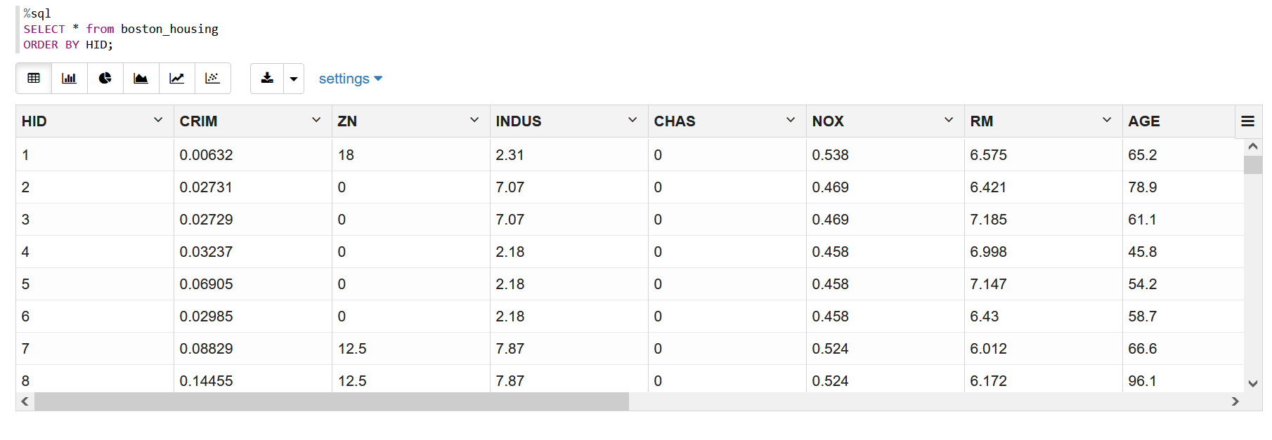
View the data in the BOSTON_HOUSING table by running the following query:
```
SELECT * FROM BOSTON_HOUSING
ORDER BY HID;
```

Since you created the table specifying each column's datatype, you already know the datatype. However, to view the datatype of the columns, run the following script:

%script
DESCRIBE BOSTON_HOUSING;


Name    Null?    Type        
------- -------- ------------
HID  NOT NULL NUMBER
CRIM          NUMBER
ZN            NUMBER
INDUS         NUMBER
CHAS          VARCHAR2(32)
NOX           NUMBER
RM            NUMBER
AGE           NUMBER
DIS           NUMBER
RAD           NUMBER(38)
TAX           NUMBER
PTRATIO       NUMBER
LSTAT         NUMBER
MEDV          NUMBER
 
---------------------------

Find the COUNT of the dataset to know how many rows are present.

SELECT COUNT (*) from BOSTON_HOUSING;


COUNT(*)   
      506
---------------------------

To check if there are any missing values (NULL values), run the following query:

SELECT COUNT(*) FROM BOSTON_HOUSING WHERE PTRATIO=NULL OR CHAS=NULL OR
 LSTAT=NULL OR TAX=NULL OR CRIM=NULL OR MEDV=NULL OR ZN=NULL OR NOX=NULL
 OR AGE=NULL OR INDUS=NULL OR DIS=NULL OR RAD=NULL OR PTRATIO=NULL OR RM=NULL;


COUNT(*)   
      0
---------------------------

NULLs, if found, are automatically handled by the OML algorithms. Alternately, you can manually replace NULLs with NVL SQL function.

To list the distinct values for the categorical column CHAS and the number of records for each distinct value of CHAS, run the following query:

%sql
SELECT CHAS, COUNT(1)
FROM BOSTON_HOUSING
GROUP BY CHAS;


CHAS   COUNT(1)   
0             471 
1              35 
---------------------------

To calculate mean, median, min, max, and interquartile range (IQR) create a view called unpivoted.

The IQR describes the middle 50% of values (also called the mid spread or the H spread) when ordered from lowest to highest. To find the IQR, first, find the median (middle value) of the lower and upper half of the data. These values are quartile 1 (Q1) and quartile 3 (Q3). The IQR is the difference between Q3 and Q1. Sometimes, this assessment is helpful to find outliers in the data.

%sql
create or replace view unpivoted as
select *
  from (
       
SELECT 'CRIM' COL, ROUND(MIN(CRIM),2) MIN_VAL, PERCENTILE_CONT(0.25) WITHIN GROUP (ORDER BY CRIM) FIRST_QUANTILE, ROUND(AVG(CRIM),2) MEAN_VAL, ROUND(MEDIAN(CRIM),2) MEDIAN_VAL, PERCENTILE_CONT(0.75) WITHIN GROUP (ORDER BY CRIM) THIRD_QUANTILE, ROUND(MAX(CRIM),2) MAX_VAL
FROM BOSTON_HOUSING
UNION
SELECT 'AGE' COL, ROUND(MIN(AGE),2) MIN_VAL,  PERCENTILE_CONT(0.25) WITHIN GROUP (ORDER BY AGE) FIRST_QUANTILE, ROUND(AVG(AGE),2) MEAN_VAL, ROUND(MEDIAN(AGE),2) MEDIAN_VAL, PERCENTILE_CONT(0.75) WITHIN GROUP (ORDER BY AGE) THIRD_QUANTILE, ROUND(MAX(AGE),2) MAX_VAL
FROM BOSTON_HOUSING
UNION
SELECT 'DIS' COL, ROUND(MIN(DIS),2) MIN_VAL,  PERCENTILE_CONT(0.25) WITHIN GROUP (ORDER BY DIS) FIRST_QUANTILE, ROUND(AVG(DIS),2) MEAN_VAL, ROUND(MEDIAN(DIS),2) MEDIAN_VAL, PERCENTILE_CONT(0.75) WITHIN GROUP (ORDER BY DIS) THIRD_QUANTILE, ROUND(MAX(DIS),2) MAX_VAL
FROM BOSTON_HOUSING
  ) a
unpivot
(
  VALUE
    for stat in ("MIN_VAL", "FIRST_QUANTILE", "MEAN_VAL","MEDIAN_VAL", "THIRD_QUANTILE", "MAX_VAL")
);

To view the values, pivot the table by running the following query:

%sql
select *
  from unpivoted
pivot(
  SUM(VALUE)
    for COL in ('CRIM', 'AGE','DIS')
);



STAT             'CRIM'      'AGE'    'DIS'      
MEAN_VAL                3.61    68.57        3.8 
THIRD_QUARTILE     3.6770825   94.075   5.188425 
MAX_VAL                88.98      100      12.13 
FIRST_QUARTILE      0.082045   45.025   2.100175 
MEDIAN_VAL              0.26     77.5       3.21 
MIN_VAL                 0.01      2.9       1.13 


6 rows selected. 

---------------------------

This completes the data understanding and data preparation stage. OML supports Automatic Data Preparation (ADP). ADP is enabled through the model settings. When ADP is enabled, the transformations required by the algorithm are performed automatically and embedded in the model. This step is done during the Build Model stage. The commonly used methods of data preparation are binning, normalization, and missing value treatment.

Related Topics

How ADP Transforms the Data

Build Model

Build your model using the training data set. Use the DBMS_DATA_MINING.CREATE_MODEL2 procedure to build your model and specify model settings.

For a supervised learning, like Regression, before creating the model, split the data in to training and test data. Although you can use the entire data set to build a model, it is difficult to validate the model unless there are new data sets available. Therefore, to evaluate the model and to accurately assess the performance of the model on the same data, you generally split or separate the data into training and test data. You use the training data set to train the model and then use the test data set to test the accuracy of the model by running prediction queries. The testing data set already contains known values for the attribute that you want to predict. It is thus easy to determine whether the model's predictions are correct.

Algorithm Selection

Before you build a model, choose the suitable algorithm. You can choose one of the following algorithms to solve a regression problem:

Extreme Gradient Boosting
Generalized Linear Model
Neural Network
Support Vector Machine

When you want to understand the data set, you always start from a simple and easy baseline model. The Generalized Linear Model algorithm is the right choice because it is simple and easy to interpret since it fits a linear relationship between the feature and the target. You can get an initial understanding of a new data set from the result of the linear model.

The following steps guide you to split your data and build your model with the selected algorithm.

Split the data into 80/20 as training and test data. Run the following statement:

BEGIN
    EXECUTE IMMEDIATE 'CREATE OR REPLACE VIEW TRAINING_DATA AS SELECT * FROM BOSTON_HOUSING SAMPLE (80) SEED (1)';
    DBMS_OUTPUT.PUT_LINE ('Created TRAINING_DATA');
    EXECUTE IMMEDIATE 'CREATE OR REPLACE VIEW TEST_DATA AS SELECT * FROM BOSTON_HOUSING MINUS SELECT * FROM TRAINING_DATA';
    DBMS_OUTPUT.PUT_LINE ('Created TEST_DATA');
    
END;

After splitting the data, view the count of rows in TRAINING_DATA and TEST_DATA. You can verify the ratio of the training and test data by checking the number of rows of the training and test set.

To find the count of rows in TRAINING_DATA, run the following statement:

select count(*) from TRAINING_DATA;

COUNT(*)
400
---------------------------

To find the count of rows from TEST_DATA, run the following statement:

select COUNT(*) from TEST_DATA;

COUNT(*)
106
---------------------------

To find if any rows are not sampled (left out) in both TRAINING_DATA and TEST_DATA, run the following query:

SELECT COUNT(1)
FROM TRAINING_DATA train
JOIN TEST_DATA test
ON train.HID = test.HID

COUNT(*)
0
---------------------------

Build your model using the CREATE_MODEL2 procedure. First, declare a variable to store model settings or hyperparameters. Run the following script:
```
%script
DECLARE
    v_setlst DBMS_DATA_MINING.SETTING_LIST;
    BEGIN
    v_setlst('PREP_AUTO') := 'ON';
    v_setlst('ALGO_NAME') := 'ALGO_GENERALIZED_LINEAR_MODEL';
    v_setlst('GLMS_DIAGNOSTICS_TABLE_NAME') := 'GLMR_DIAG';
    v_setlst('GLMS_FTR_SELECTION') := 'GLMS_FTR_SELECTION_ENABLE';
    v_setlst('GLMS_FTR_GENERATION') := 'GLMS_FTR_GENERATION_ENABLE';
     
    DBMS_DATA_MINING.CREATE_MODEL2(
      MODEL_NAME          =>  'GLMR_REGR',
      MINING_FUNCTION     => 'REGRESSION'
      DATA_QUERY          =>  'SELECT * FROM TRAINING_DATA',
      SET_LIST            =>  v_setlst,
      CASE_ID_COLUMN_NAME =>  'HID',
      TARGET_COLUMN_NAME  =>  'MEDV');
END;
```
Examine the script:
- v_setlst is a variable to store SETTING_LIST.
- SETTING_LIST defines model settings or hyperparameters for your model.
- DBMS_DATA_MINING is the PL/SQL package used for Oracle Machine Learning. These settings are described in DBMS_DATA_MINING - Model Settings.
- ALGO_NAME specifies the algorithm name. Since you are using the Generalized Linear Model as your algorithm, set ALGO_GENERALIZED_LINEAR_MODEL.
- PREP_AUTO is the setting used for Automatic Data Preparation. Here, enable Automatic Data Preparation. The value of the setting is ON.
- GLMS_DIAGNOSTICS_TABLE_NAME generates per-row statistics if you specify the name of a diagnostics table in the setting. The value of the setting is GLMR_DIAG.
- GLMS_FTR_SELECTION indicates feature selection. The value GLMS_FTR_SELECTION_ENABLE indicates that feature selection is enabled. Feature selection selects columns that are most important in predicting a target attribute. If feature selection is not selected, then all the columns are considered for analysis which may not give accurate results.
- GLMS_FTR_GENERATION indicates feature generation. The value GLMS_FTR_GENERATION_ENABLE indicates that the feature generation is enabled. Feature generation generates new features from existing features which might be useful in our analysis.
The CREATE_MODEL2 procedure has the following parameters:
- MODEL_NAME: A unique model name that you want to give to your model. The name of the model is in the form [schema_name.]model_name. If you do not specify a schema, then your own schema is used. Here, the model name is GLMR_REGR
- MINING_FUNCTION: Specifies the machine learning function. Since you are solving a linear regression problem, in this use case, select REGRESSION.
- DATA_QUERY: A query that provides training data for building the model. Here, the query is SELECT * FROM TRAINING_DATA.
- SET_LIST: Specifies SETTING_LIST.
- CASE_ID_COLUMN_NAME: A unique case identifier column in the training data. In this use case, case_id is HID. If there is a composite key, you must create a new attribute before creating the model. The CASE_ID assists with reproducible results, joining scores for individual customers with other data in, example, scoring data table.
- TARGET_COLUMN_NAME: Specifies the column that needs to be predicted. Also referred to as the target variable of the model. In this use case, you are predicting MEDV value.
Note:
Any parameters or settings not specified are either system-determined or default values are used.

Evaluate

Evaluate your model by viewing diagnostic metrics and performing quality checks.

Sometimes querying dictionary views and model detail views is sufficient to measure your model's performance. However, you can evaluate your model by computing test metrics such as Mean Absolute Error (MAE), Root Mean Squared Error (RMSE), confusion matrix, lift statistics, cost matrix, and so on. For Association Rules, you can inspect various rules to see if they reveal new insights for item dependencies (antecedent itemset implying consequent) or for unexpected relationships among items.

Dictionary and Model Views

To obtain information about the model and view model settings, you can query data dictionary views and model detail views. Specific views in model detail views display model statistics which can help you evaluate the model.

The data dictionary views for Oracle Machine Learning are listed in the following table. A database administrator (DBA) and USER versions of the views are also available.

View Name	Description
ALL_MINING_MODELS	Provides information about all accessible machine learning models
ALL_MINING_MODEL_ATTRIBUTES	Provides information about the attributes of all accessible machine learning models
ALL_MINING_MODEL_SETTINGS	Provides information about the configuration settings for all accessible machine learning models
ALL_MINING_MODEL_VIEWS	Provides information about the model views for all accessible machine learning models
ALL_MINING_MODEL_XFORMS	Provides the user-specified transformations embedded in all accessible machine learning models.

Model detail views are specific to the algorithm. You can obtain more insights about the model you created by viewing the model detail views. The names of model detail views begin with DM$xx where xx corresponds to the view prefix. See Model Detail Views.

The following steps help you to view different dictionary views and model detail views.

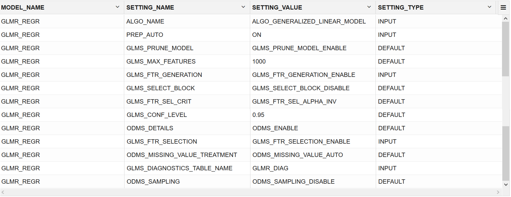
Run the following statement to view the settings in USER_MINING_MODEL_SETTINGS:
```
SELECT * FROM USER_MINING_MODEL_SETTINGS WHERE MODEL_NAME='GLMR_REGR';
```
In this statement, you are selecting all the columns available in the USER_MINING_MODEL_SETTINGS view where the model name is GLMR_REGR.

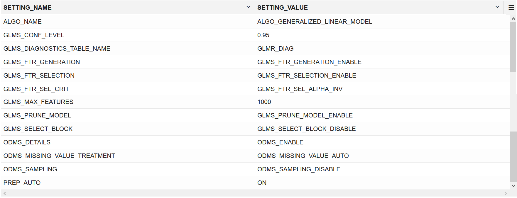
Run the following statement to view only the SETTING_NAME and SETTING_VALUE column from the above table:

SELECT SETTING_NAME, SETTING_VALUE FROM USER_MINING_MODEL_SETTINGS WHERE MODEL_NAME = 'GLMR_REGR' ORDER BY SETTING_NAME;

Run the following statement to see attribute information in USER_MINING_MODEL_ATTRIBUTES view:

SELECT ATTRIBUTE_NAME, ATTRIBUTE_TYPE FROM USER_MINING_MODEL_ATTRIBUTES WHERE MODEL_NAME = 'GLMR_REGR' ORDER BY ATTRIBUTE_NAME;

Run the following statement to see information on various views in USER_MINING_MODEL_VIEWS:

SELECT VIEW_NAME, VIEW_TYPE FROM USER_MINING_MODEL_VIEWS WHERE MODEL_NAME='GLMR_REGR' ORDER BY VIEW_NAME;

From the table above, query the Global details for linear regression. See Model Detail Views for Generalized Linear Model. Run the following query to see all the columns of the view:
```
SELECT * FROM DM$VGGLMR_REGR;
```
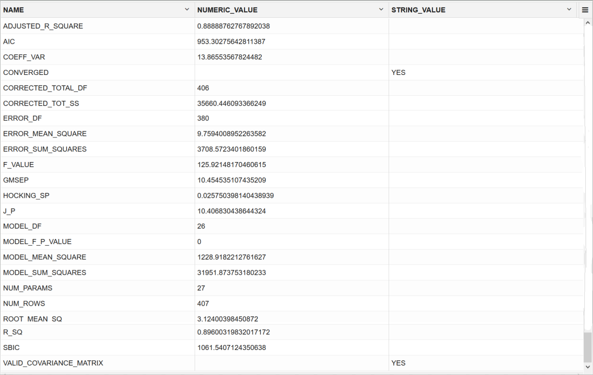
From the above table, you can ignore the first column PARTITION_NAME and refine the query to display the rest of the columns ordered by name. Run the following statement:
```
SELECT NAME, NUMERIC_VALUE, STRING_VALUE FROM DM$VGGLMR_REGR ORDER BY NAME;
```
When comparing models, a model with a lower Root Mean Square Error (RMSE) value is better. RMSE, which squares the errors, gives more weight to large errors. When we have a low RMSE value, we can say that our model is good at predicting the target.
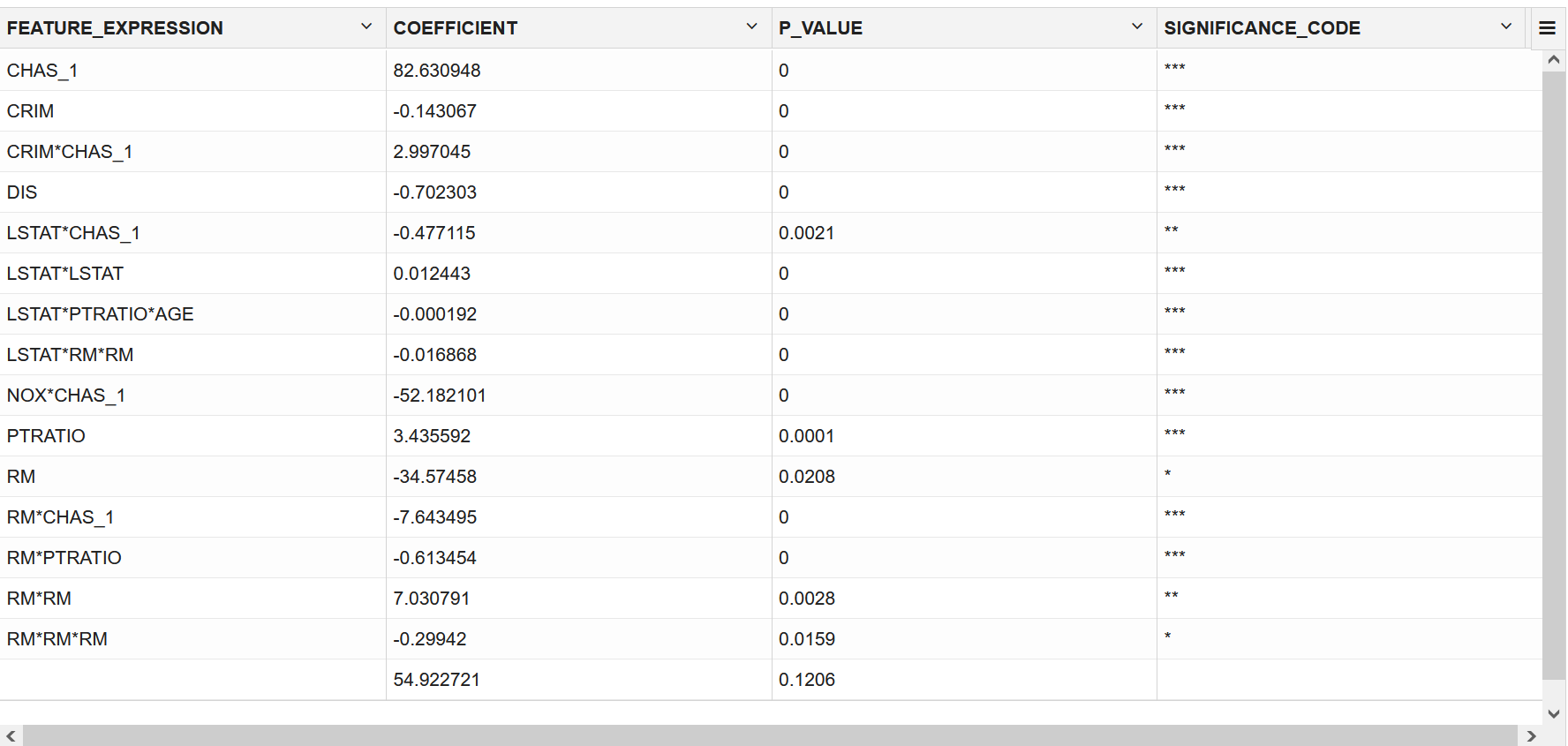
Query the GLM Regression Attributes Diagnostics view.
```
SELECT FEATURE_EXPRESSION, round(COEFFICIENT,6) COEFFICIENT, round(P_VALUE,4) P_VALUE,
CASE
    when p_value < 0.001 THEN '***'
    when p_value < 0.01 THEN '**'
    when p_value < 0.05 THEN '*'
    when p_value < 0.1 THEN '.'
    else ' '
END AS significance_statement
FROM DM$VDGLMR_REGR ORDER BY FEATURE_EXPRESSION;
```
The columns of the view are described in Model Detail Views for Generalized Linear Model.
Let us examine the statement:
- round(COEFFICIENT,6) COEFFICIENT: returns the coefficient rounded to six places to the right of the decimal point.
- p_value: provides information about the relationship between a dependent variable and independent variable such that you could decide to accept or reject the null hypothesis. Generally, p_value less than 0.05 means that you can reject the null hypothesis and accept that there is a correlation between the dependent and independent variables with a significant coefficient value.
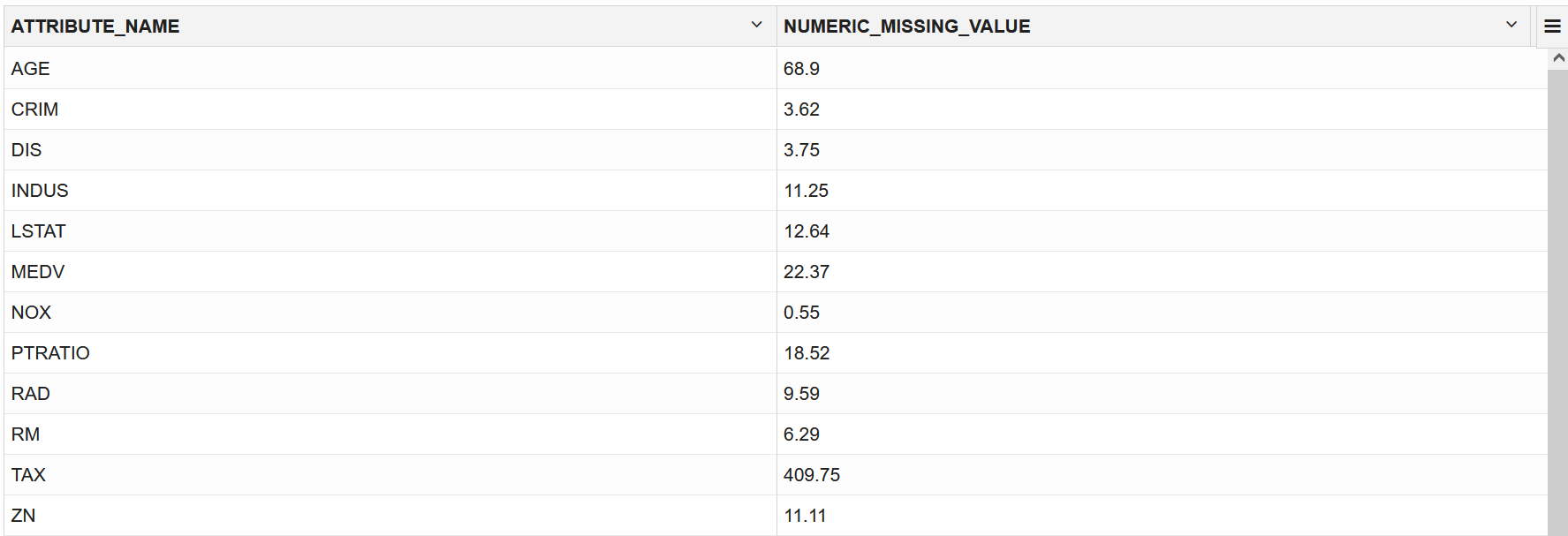
Now, run the following statement to query Normalization and Missing Value Handling view. The columns of the view are described in Model Detail Views for Normalization and Missing Value Handling.
```
SELECT ATTRIBUTE_NAME, round(NUMERIC_MISSING_VALUE,2) NUMERIC_MISSING_VALUE FROM DM$VNGLMR_REGR
ORDER BY ATTRIBUTE_NAME;
```
Examine the query:
- ATTRIBUTE_NAME: Provides the column names in the data set.
- round(NUMERIC_MISSING_VALUE,2)NUMERIC_MISSING_VALUE: Provides numeric replacements for the missing values (NULLs) in the data set. The ROUND (n,integer) returns results of NUMERIC_MISSING_VALUE rounded to integer places to the right.
Since there are no missing values (NULLs) in your data, you can ignore the result.

Test Your Model

In this use case, you are evaluating a regression model by computing Root Mean Square Error (RMSE) and Mean Absolute Error Mean (MAE) on the test data with known target values and comparing the predicted values with the known values.

Test metrics are used to assess how accurately the model predicts the known values. If the model performs well and meets your business requirements, it can then be applied to new data to predict the future. These matrices can help you to compare models to arrive at one model that satisfies your evaluation criteria.

For this use case, you compute Root Mean Square Error (RMSE) and Mean Absolute Error Mean (MAE) values. The RMSE and MAE are popular regression statistics. RMSE is an estimator for predictive models. The score averages the residuals for each case to yield a single indicator of model error. Mean absolute error is useful for understanding how close overall the predictions were to actual values. A smaller score means predictions were more accurate.

The following steps computes the error metrics for your model.

To compute RMSE and MAE, run the following statement:

%sql
SELECT round(SQRT(AVG((A.PRED_MEDV - B.MEDV) * (A.PRED_MEDV - B.MEDV))),2) RMSE,
       round(AVG(ABS(A.PRED_MEDV - B.MEDV)),2) MAE
  FROM (SELECT HID, PREDICTION(GLMR_REGR using *) PRED_MEDV
          FROM TEST_DATA) A,
       TEST_DATA B
  WHERE A.HID = B.HID;

This statement is using the prediction query to score the median value from the test data. The predicted value and the actual value from the test data is used to compute RMSE and MAE .

RMSE and MAE convey average model prediction errors in units consistent with the target variable. When comparing models, a model with lower values is better. RMSE, which squares the errors, gives more weight to large errors, while MAE error scales linearly. Therefore, the predictions look fair and the model is a good fit for prediction.

Score

Scoring involves applying the model to the target data. Use PREDICTION query to predict the MEDV value on the test data.

The following step scores the test data comparing with the original data.

Predict the median value of owner-occupied homes in the Boston area from the TEST_DATA and compare the predicted MEDV value with the actual MEDV value in your result.
```
SELECT HID, ROUND(PREDICTION(GLMR_REGR USING *), 1) AS 
PREDICTED_MEDV, MEDV AS ACTUAL_MEDV FROM TEST_DATA ORDER BY HID;
```
Examine the query:
- HID: is the House ID.
- ROUND (n,integer): in this case, is ROUND (PREDICTION(GLMR_REGR USING *), 1) returns results of PREDICTION(GLMR_REGR USING *) rounded to integer places to the right. Here, rounded to 1 place to the right.
- PREDICTED_MEDV: is the predicted MEDV value.
- ACTUAL_MEDV: is the MEDV value in the test data.

To conclude, you have successfully predicted the median house prices in Boston using Generalized Linear Model algorithm.