Classification Use Case Scenario

You are working in a retail chain company that sells some products. To better target their marketing materials, they need to identify customers who are likely to purchase a home theater package. To resolve this, you are using the Random Forest algorithm to identify the customers.

Related Content

Topic	Link
OML4SQL GitHub Example	Classification - Random Forest
CREATE_MODEL2 Procedure	CREATE_MODEL2 Procedure
Generic Model Settings	DBMS_DATA_MINING - Model Settings
Random Forest Settings	DBMS_DATA_MINING - Algorithm Settings: Random Forest
Data Dictionary Settings	Oracle Machine Learning Data Dictionary Views
Random Forest - Model Detail Views	Model Detail Views for Random Forest
About Classification	About Classification
About Random Forest (RF)	About Random Forest

Before you start your OML4SQL use case journey, ensure that you have the following:

• Data Set

  The data set used for this use case is from the SH schema. The SH schema can be readily accessed in Oracle Autonomous Database. For on-premises databases, the schema is installed during the installation or can be manually installed by downloading the scripts. See Installing the Sample Schemas.

• Database
  Select or create database out of the following options:

  • Get your FREE cloud account. Go to https://cloud.oracle.com/database and select Oracle Database Cloud Service (DBCS), or Oracle Autonomous Database. Create an account and create an instance. See Autonomous Database Quick Start Workshop.
  • Download the latest version of Oracle Database (on premises).
• Machine Learning Tools
  Depending on your database selection,

  • Use OML Notebooks for Oracle Autonomous Database.
  • Install and use Oracle SQL Developer connected to an on-premises database or DBCS. See Installing and Getting Started with SQL Developer.
• Other Requirements

  Data Mining Privileges (this is automatically set for ADW). See System Privileges for Oracle Machine Learning for SQL.

Load Data

Access the data set from the SH Schema and explore the data to understand the attributes.

Remember:

The data set used for this use case is from the SH schema. The SH schema can be readily accessed in Oracle Autonomous Database. For on-premises databases, the schema is installed during the installation or can be manually installed by downloading the scripts. See Installing the Sample Schemas.

To understand the data, you will perform the following:

• Access the data.
• Examine the various attributes or columns of the data set.
• Assess data quality (by exploring the data).

Access Data

You will use CUSTOMERS and SUPPLEMENTARY_DEMOGRAPHICS table data from the SH schema.

Examine Data

The following table displays information about the attributes from SUPPLEMENTARY_DEMOGRAPHICS:

Attribute Name	Information
CUST_ID	The ID of the customer
EDUCATION	Educational information of the customer
OCCUPATION	Occupation of the customer
HOUSEHOLD_SIZE	People per house
YRS_RESIDENCE	Number of years of residence
AFFINITY_CARD	Whether the customer holds an affinity card
BULK_PACK_DISKETTES	Product. Indicates whether the customer already owns the product. 1 means Yes. 0 means No
FLAT_PANEL_MONITOR	Product. Indicates whether the customer already owns the product. 1 means Yes. 0 means No
HOME_THEATER_PACKAGE	Product. Indicates whether the customer already owns the product. 1 means Yes. 0 means No
BOOKKEEPING_APPLICATION	Product. Indicates whether the customer already owns the product. 1 means Yes. 0 means No
PRINTER_SUPPLIES	Product. Indicates whether the customer already owns the product. 1 means Yes. 0 means No
Y_BOX_GAMES	Product. Indicates whether the customer already owns the product. 1 means Yes. 0 means No
OS_DOC_SET_KANJI	Product. Indicates whether the customer already owns the product. 1 means Yes. 0 means No
COMMENTS	Product. Indicates whether the customer already owns the product. 1 means Yes. 0 means No

Explore Data

Explore the data to understand and assess the quality of the data. At this stage assess the data to identify data types and noise in the data. Look for missing values and numeric outlier values.

Assess Data Quality

To assess the data, first, you must be able to view the data in your database. For this reason, you will use SQL statements to query the SH.CUSTOMERS and the SH.SUPPLEMENTARY_DEMOGRAPHICS table.

If you are working with Oracle Autonomous Database, you can use the Oracle Machine Learning (OML) Notebooks for your data science project, including assessing data quality. If you are using on-premise Oracle Database, you can use the Oracle SQL Developer to assess data quality. Query the SH schema as described.

Note:

Each record in the database is called a case and each case is identified by a case_id. In this use case, CUST_ID is the case_id.

1. View the data in the SH.CUSTOMERS table by running the following statement:

   SELECT * FROM SH.CUSTOMERS;

2. To see distinct data from the table, run the following statement:

   SELECT DISTINCT * FROM SH.CUSTOMERS;

   
3. Find the COUNT of rows in the data set by running the following statement:

   SELECT COUNT(*) from SH.CUSTOMERS;

   
   COUNT(*)   
        55500 
   ---------------------------

4. To identify distinct or unique customers in the table, run the following statement:

   
   %script
   SELECT COUNT (DISTINCT CUST_ID) FROM SH.CUSTOMERS; 

   
   COUNT(DISTINCTCUST_ID)   
                      55500 
   ---------------------------

5. Similarly, query the SH.SUPPLEMENTARY_DEMOGRAPHICS table.

   SELECT * FROM SH.SUPPLEMENTARY_DEMOGRAPHICS;

   
6. To view the count of SH.SUPPLEMENTARY_DEMOGRAPHICS, run the following statement:

   SELECT COUNT(*) from SH.SUPPLEMENTARY_DEMOGRAPHICS;
   

   
   COUNT(*)   
         4500 
   ---------------------------
   

7. Create a table called CUSTOMERDATA by selecting the required columns from the SH.CUSTOMERS and the SH.SUPPLIMENTARY_DEMOGRAPHICS tables.

   %script
   CREATE TABLE CUSTOMERDATA AS
      SELECT a.CUST_ID,
            a.CUST_INCOME_LEVEL, a.CUST_CREDIT_LIMIT,
             b.HOUSEHOLD_SIZE, b.OCCUPATION, b.HOME_THEATER_PACKAGE
      FROM SH.CUSTOMERS a, SH.SUPPLEMENTARY_DEMOGRAPHICS b
      WHERE a.CUST_ID = b.CUST_ID;
    

   
   Table CUSTOMERDATA created.

8. View the CUSTOMERDATA table.

   SELECT * FROM CUSTOMERDATA;

   
9. Find the count of rows in the new table CUSTOMERDATA:

   SELECT COUNT(*) FROM CUSTOMERDATA;

   
   COUNT(*)   
         4500 
   ---------------------------

10. To view the data type of the columns, run the following script:

    %script
    DESCRIBE CUSTOMERDATA;
    

    
    Name                Null?    Type        
    ------------------- -------- ------------
    CUST_ID       	   NOT NULL  NUMBER
    CUST_GENDER 	   NOT NULL  CHAR(1)
    CUST_MARITAL_STATUS          VARCHAR2(20)
    CUST_YEAR_OF_BIRTH NOT NULL  NUMBER(4)
    CUST_INCOME_LEVEL            VARCHAR2(30)
    CUST_CREDIT_LIMIT            NUMBER
    HOUSEHOLD_SIZE          	 VARCHAR2(21)
    YRS_RESIDENCE          		 NUMBER
    Y_BOX_GAMES          		 NUMBER(10)
     
    ---------------------------

11. To check if there are any missing values (NULL values), run the following statement:

    SELECT COUNT(*) FROM CUSTOMERDATA WHERE CUST_ID=NULL OR CUST_GENDER=NULL
     OR CUST_MARITAL_STATUS=NULL OR CUST_YEAR_OF_BIRTH=NULL OR CUST_INCOME_LEVEL=NULL
     OR CUST_CREDIT_LIMIT=NULL OR HOUSEHOLD_SIZE=NULL OR YRS_RESIDENCE=NULL OR Y_BOX_GAMES=NULL;
    
    

    
    COUNT(*)   
             0 
    ---------------------------

    NULLs, if found, are automatically handled by the OML algorithms. Alternately, you can manually replace NULLs with NVL SQL function.

12. To know the income level of customers who responded to HOME_THEATER_PACKAGE, run the following statement:

    SELECT COUNT(CUST_ID) AS NUM_CUSTOMERS, CUST_INCOME_LEVEL, HOME_THEATER_PACKAGE
    FROM   CUSTOMERDATA
    GROUP BY CUST_INCOME_LEVEL, HOME_THEATER_PACKAGE;
    

    
    NUM_CUSTOMERS   CUST_INCOME_LEVEL      HOME_THEATER_PACKAGE   
                214 K: 250,000 - 299,999                        0 
                315 L: 300,000 and above                        1 
                114 E: 90,000 - 109,999                         0 
                 27 A: Below 30,000                             0 
                 61 A: Below 30,000                             1 
                206 F: 110,000 - 129,999                        1 
                446 J: 190,000 - 249,999                        0 
                196 E: 90,000 - 109,999                         1 
                 90 B: 30,000 - 49,999                          0 
                 99 C: 50,000 - 69,999                          1 
                319 I: 170,000 - 189,999                        1 
                165 I: 170,000 - 189,999                        0 
                179 K: 250,000 - 299,999                        1 
                142 H: 150,000 - 169,999                        0 
    
    NUM_CUSTOMERS   CUST_INCOME_LEVEL      HOME_THEATER_PACKAGE   
                163 F: 110,000 - 129,999                        0 
                 83 D: 70,000 - 89,999                          1 
                 50 D: 70,000 - 89,999                          0 
                328 L: 300,000 and above                        0 
                519 J: 190,000 - 249,999                        1 
                189 G: 130,000 - 149,999                        1 
                150 G: 130,000 - 149,999                        0 
                132 B: 30,000 - 49,999                          1 
                 72 C: 50,000 - 69,999                          0 
                241 H: 150,000 - 169,999                        1 
    
    
    24 rows selected. 
    ---------------------------

This completes the data exploration stage. OML supports Automatic Data Preparation (ADP). ADP is enabled through the model settings. When ADP is enabled, the transformations required by the algorithm are performed automatically and embedded in the model. This step is done during the Build Model stage. The commonly used methods of data preparation are binning, normalization, and missing value treatment.

Build Model

Build your model using the training data set. Use the DBMS_DATA_MINING.CREATE_MODEL2 procedure to build your model and specify the model settings.

For a supervised learning, like Classification, before creating the model, split the data into training and test data. Although you can use the entire data set to build a model, it is difficult to validate the model unless there are new data sets available. Therefore, to evaluate the model and to accurately assess the performance of the model on the same data, you generally split or separate the data into training and test data. You use the training data set to train the model and then use the test data set to test the accuracy of the model by running prediction queries. The testing data set already contains known values for the attribute that you want to predict. It is thus easy to determine whether the predictions of the model are correct.

Algorithm Selection

Before you build a model, choose the suitable algorithm. You can choose one of the following algorithms to solve a classification problem:

• Decision Tree
• Explicit Semantic Analysis (ESM)
• Generalized Linear Model (GLM)
• Naive Bayes
• Random Forest
• Support Vector Machine (SVM)
• XGBoost

From the above algorithms, ESM is more about Natural Language Processing (NLP) and text mining. ESM does not apply to this use case and data. If you were to select a relatively simple linear model like GLM, the prediction accuracy can be further improved by the Random Forest algorithm. Random Forest is an ensemble method that builds multiple decision trees on subsets of the data re-sampled at each time (bagging). This avoids the overfitting for a single decision tree. The random forest model is a widely used ensemble method that is known to have higher accuracy than linear models. Thus, Random Forest is selected for this use case.

For this use case, split the data into 60/40 as training and test data. You build the model using the training data and once the model is built, score the test data using the model.

The following steps guide you to split your data and build your model with the selected algorithm.

1. To create the training and test data with 60/40 split, run the following statement:

   CREATE OR REPLACE VIEW TRAINING_DATA AS SELECT * FROM CUSTOMERDATA SAMPLE (60) SEED (1);
   --DBMS_OUTPUT.PUT_LINE ('Created TRAINING_DATA');
   CREATE OR REPLACE VIEW TEST_DATA AS SELECT * FROM CUSTOMERDATA MINUS SELECT * FROM TRAINING_DATA;
   --DBMS_OUTPUT.PUT_LINE ('Created TEST_DATA');
    

   
   View TRAINING_DATA created.
   ---------------------------
   View TEST_DATA created.

2. To view the data in the training_data view, run the following statement:

   SELECT * FROM TRAINING_DATA;

   
3. To view the data in the test_data view, run the following statement:

   SELECT* FROM TEST_DATA;

   
4. To view the distribution of HOME_THEATER_PACKAGE (target) owners, run the following script:

   %script
   select HOME_THEATER_PACKAGE, count(1)
   from training_data
   group by HOME_THEATER_PACKAGE;

   
   HOME_THEATER_PACKAGE   COUNT(1)   
                        1       1506 
                        0       1208 
   
   ---------------------------

5. Build your model using the CREATE_MODEL2 procedure. First, declare a variable to store model settings or hyperparameters. Run the following script:

   %script
    
   BEGIN DBMS_DATA_MINING.DROP_MODEL('MODEL_RF');
   EXCEPTION WHEN OTHERS THEN NULL; END;
   /
   DECLARE
       v_setlist DBMS_DATA_MINING.SETTING_LIST;
        
   BEGIN
       v_setlist('PREP_AUTO') := 'ON';
       v_setlist('ALGO_NAME') := 'ALGO_RANDOM_FOREST';
       v_setlist('RFOR_NUM_TREES') := '25';
        
       DBMS_DATA_MINING.CREATE_MODEL2(
         MODEL_NAME          =>  'MODEL_RF',
         MINING_FUNCTION     => 'CLASSIFICATION',
         DATA_QUERY          =>  'SELECT * FROM TRAINING_DATA',
         SET_LIST            =>  v_setlist,
         CASE_ID_COLUMN_NAME =>  'CUST_ID',
         TARGET_COLUMN_NAME  =>  'HOME_THEATER_PACKAGE');
   END;
    

   
   PL/SQL procedure successfully completed.
   
   ---------------------------
    
   PL/SQL procedure successfully completed.

   Examine the script:

   • v_setlist is a variable to store SETTING_LIST.
   • SETTING_LIST defines model settings or hyperparameters for your model.
   • DBMS_DATA_MINING is the PL/SQL package used for machine learning. These settings are described in DBMS_DATA_MINING - Model Settings.
   • ALGO_NAME specifies the algorithm name. Since you are using Random Forest as the algorithm, set ALGO_RANDOM_FOREST.
   • PREP_AUTO is the setting used for Automatic Data Preparation. Here, enable Automatic Data Preparation. The value of the setting is ON.
   • RFOR_NUM_TREES is the number of trees in the forest. The value here is 25. Random forest resolves the overfitting problem by training multiple trees on distinct sampled subsets of the data instead of on the same, entire training set. The more trees you select, the more accuracy it can obtain. However, keep in mind that more trees mean more computation load and longer model building time. You need to do a trade-off between the time cost and model accuracy here. Choosing the number of trees equal to 25 allows you to build the model in a reasonably short time and obtain an accurate enough model.

   The CREATE_MODEL2 procedure takes the following parameters:

   • MODEL_NAME: A unique model name that you will give to the model. The name of the model is in the form [schema_name.]model_name. If you do not specify a schema, then your own schema is used. Here, the model name is MODEL_RF

   • MINING_FUNCTION: Specifies the machine learning function. Since it is a classification problem in this use case, select CLASSIFICATION.

   • DATA_QUERY: A query that provides training data for building the model. Here, the query is SELECT * FROM TRAINING_DATA.

   • SET_LIST: Specifies SETTING_LIST.

   • CASE_ID_COLUMN_NAME: A unique case identifier column in the build data. In this use case, case_id is CUST_ID. If there is a composite key, you must create a new attribute before creating the model. The CASE_ID assists with reproducible results, joining scores for individual customers with other data in, example, scoring data table.

   Note:

   Any parameters or settings not specified are either system-determined or default values are used.

Evaluate

Evaluate your model by viewing diagnostic metrics and performing quality checks.

Sometimes querying dictionary views and model detail views is sufficient to measure your model's performance. However, you can evaluate your model by computing test metrics such as Mean Absolute Error (MAE), Root Mean Squared Error (RMSE), confusion matrix, lift statistics, cost matrix, and so on. For Association Rules, you can inspect various rules to see if they reveal new insights for item dependencies (antecedent itemset implying consequent) or for unexpected relationships among items.

Dictionary and Model Views

To obtain information about the model and view model settings, you can query data dictionary views and model detail views. Specific views in model detail views display model statistics which can help you evaluate the model.

The data dictionary views for Oracle Machine Learning are listed in the following table. A database administrator (DBA) and USER versions of the views are also available.

View Name	Description
ALL_MINING_MODELS	Provides information about all accessible machine learning models
ALL_MINING_MODEL_ATTRIBUTES	Provides information about the attributes of all accessible machine learning models
ALL_MINING_MODEL_SETTINGS	Provides information about the configuration settings for all accessible machine learning models
ALL_MINING_MODEL_VIEWS	Provides information about the model views for all accessible machine learning models
ALL_MINING_MODEL_XFORMS	Provides the user-specified transformations embedded in all accessible machine learning models.

Model detail views are specific to the algorithm. You can obtain more insights about the model you created by viewing the model detail views. The names of model detail views begin with DM$xx where xx corresponds to the view prefix. See Model Detail Views.

The following steps help you to view different dictionary views and model detail views.

1. Run the following statement to view the settings in USER_MINING_MODEL_SETTINGS:

   %script
   
   SELECT SETTING_NAME, SETTING_VALUE 
     FROM USER_MINING_MODEL_SETTINGS
     WHERE MODEL_NAME='MODEL_RF'
     ORDER BY SETTING_NAME;

   
   SETTING_NAME                   SETTING_VALUE             
   ALGO_NAME                      ALGO_RANDOM_FOREST        
   CLAS_MAX_SUP_BINS              32                        
   CLAS_WEIGHTS_BALANCED          OFF                       
   ODMS_DETAILS                   ODMS_ENABLE               
   ODMS_MISSING_VALUE_TREATMENT   ODMS_MISSING_VALUE_AUTO   
   ODMS_RANDOM_SEED               0                         
   ODMS_SAMPLING                  ODMS_SAMPLING_DISABLE     
   PREP_AUTO                      ON                        
   RFOR_NUM_TREES                 25                        
   RFOR_SAMPLING_RATIO            .5                        
   TREE_IMPURITY_METRIC           TREE_IMPURITY_GINI        
   TREE_TERM_MAX_DEPTH            16                        
   TREE_TERM_MINPCT_NODE          .05                       
   TREE_TERM_MINPCT_SPLIT         .1                        
   
   SETTING_NAME             SETTING_VALUE   
   TREE_TERM_MINREC_NODE    10              
   TREE_TERM_MINREC_SPLIT   20              
   
   
   16 rows selected. 
   ---------------------------

2. Run the following statement to see attribute information in USER_MINING_MODEL_ATTRIBUTES view:

   %script
   SELECT ATTRIBUTE_NAME, ATTRIBUTE_TYPE 
   FROM USER_MINING_MODEL_ATTRIBUTES 
   WHERE MODEL_NAME = 'MODEL_RF' 
   ORDER BY ATTRIBUTE_NAME;

   
   ATTRIBUTE_NAME         ATTRIBUTE_TYPE   
   CUST_CREDIT_LIMIT      NUMERICAL        
   HOME_THEATER_PACKAGE   CATEGORICAL      
   HOUSEHOLD_SIZE         CATEGORICAL      
   OCCUPATION             CATEGORICAL      
   
   ---------------------------

3. Run the following statement to view various model detail views from USER_MINING_MODEL_VIEWS:

   %script
   SELECT VIEW_NAME, VIEW_TYPE
     FROM USER_MINING_MODEL_VIEWS
     WHERE MODEL_NAME='MODEL_RF'
     ORDER BY VIEW_NAME;

   
   VIEW_NAME       VIEW_TYPE                 
   DM$VAMODEL_RF   Variable Importance       
   DM$VCMODEL_RF   Scoring Cost Matrix       
   DM$VGMODEL_RF   Global Name-Value Pairs   
   DM$VSMODEL_RF   Computed Settings         
   DM$VTMODEL_RF   Classification Targets    
   DM$VWMODEL_RF   Model Build Alerts        
   
   
   6 rows selected. 
   ---------------------------

4. Now, view the Classification targets view. This view describes the target (HOME_THEATER_PACKAGE) distribution for classification models.

   %script
   SELECT* from DM$VTMODEL_RF;

   
   PARTITION_NAME   TARGET_VALUE   TARGET_COUNT   TARGET_WEIGHT   
                                 0           1178                 
                                 1           1549                 
   
   ---------------------------

   The distribution value from this view validates the earlier target distribution that was obtained from the training data. The difference in the values is minimal.

Test Your Model

In this use case, you are evaluating a classification model by computing Lift and Confusion Matrix on the test data with known target values and comparing the predicted values with the known values.

Test metrics are used to assess how accurately the model predicts the known values. If the model performs well and meets your business requirements, it can then be applied to new data to predict the future. These matrices can help you to compare models to arrive at one model that satisfies your evaluation criteria.

Lift measures the degree to which the predictions of a classification model are better than randomly-generated predictions. Lift can be understood as a ratio of two percentages: the percentage of correct positive classifications made by the model to the percentage of actual positive classifications in the test data.

A confusion matrix displays the number of correct and incorrect predictions made by the model compared with the actual classifications in the test data. The matrix is n-by-n, where n is the number of classes.

1. Create a result table to store the predictions for each row with likely and unlikely probabilities. Run the following script:

   %script
    
   BEGIN EXECUTE IMMEDIATE 'DROP TABLE APPLY_RESULT PURGE';
   EXCEPTION WHEN OTHERS THEN NULL; END;
   /
    
   CREATE TABLE APPLY_RESULT AS
       SELECT cust_id, t.prediction, t.probability
       FROM TEST_DATA, TABLE(PREDICTION_SET(MODEL_RF USING *)) t;
    

   
   PL/SQL procedure successfully completed.
   ---------------------------
   Table APPLY_RESULT created.
   ---------------------------

   Examine the script:

   APPLY_RESULT: is a table that stores the results of the prediction.

   TABLE(PREDICTION_SET(MODEL_RF USING *)): is a table that has results from the PREDICTION_SET query. The PREDICTION_SET query returns probabilities for each row.

2. Compute lift by using the DBMS_DATA_MINING.APPLY and the DBMS_DATA_MINING.COMPUTE_LIFT procedures:

   %script
    
   BEGIN EXECUTE IMMEDIATE 'DROP TABLE APPLY_RESULT PURGE';
   EXCEPTION WHEN OTHERS THEN NULL; END;
   /
    
   BEGIN
     DBMS_DATA_MINING.APPLY('MODEL_RF','TEST_DATA','CUST_ID','APPLY_RESULT');
      
                                     
        
          DBMS_DATA_MINING.COMPUTE_LIFT (
             apply_result_table_name           => 'APPLY_RESULT',
             target_table_name                  => 'TEST_DATA',
             case_id_column_name               => 'CUST_ID',
             target_column_name                 => 'HOME_THEATER_PACKAGE',
             lift_table_name                       => 'LIFT_TABLE',
             positive_target_value           =>  to_char(1),
             score_column_name                  => 'PREDICTION',
             score_criterion_column_name    => 'PROBABILITY',
             num_quantiles                       =>  10,
             cost_matrix_table_name             =>  null,
             apply_result_schema_name         =>  null,
             target_schema_name                 =>  null,
             cost_matrix_schema_name           =>  null,
             score_criterion_type             =>  'PROBABILITY');
        
                                     
   END;
    

   
   PL/SQL procedure successfully completed.
   ---------------------------
   PL/SQL procedure successfully completed.

   Examine the script:

   • DBMS_DATA_MINING.APPLY: This procedure creates a table in the user's schema to hold the results. The APPLY procedure generates predictions (scores) in a target column.

     The APPLY procedure has the following parameters:

     • model_name: Name of the model in the form [schema_name.]model_name. If you do not specify a schema, then your own schema is used. Here, the model name is MODEL_RF.
     • data_table_name: Name of table or view containing the data to be scored. Here, you are using TEST_DATA.
     • case_id_column_name: Name of the case identifier column. The case ID is CUST_ID.
     • result_table_name: Name of the table in which to store apply results. Here, the result table name is APPLY_RESULT.
   • DBMS_DATA_MINING.COMPUTE_LIFT: This procedure computes lift and stores them in the user's schema. To compute lift, one of the target values must be designated as the positive class.
     The COMPUTE_LIFT procedure has the following parameters:

     • apply_result_table_name: Table containing the predictions. For this use case, it is APPLY_RESULT.
     • target_table_name: Table containing the known target values from the test data. In this use case, the target table name is TEST_DATA.
     • case_id_column_name: Case ID column in the apply results table. Must match the case identifier in the targets table. The case ID column is CUST_ID.
     • target_column_name: Target column in the targets table. Contains the known target values from the test data. In this use case, the target is HOME_THEATER_PACKAGE.
     • lift_table_name: Table containing the lift statistics. The table will be created by the procedure in the user's schema. Type LIFT_TABLE.
     • positive_target_value: The positive class. This should be the class of interest, for which you want to calculate lift. If the target column is a NUMBER, you can use the TO_CHAR() operator to provide the value as a string.
     • score_column_name: Column containing the predictions in the apply results table. The default column name is 'PREDICTION', which is the default name created by the APPLY procedure.
     • score_criterion_column_name: Column containing the scoring criterion in the apply results table. Contains either the probabilities or the costs that determine the predictions. By default, scoring is based on probability; the class with the highest probability is predicted for each case. If scoring is based on cost, the class with the lowest cost is predicted. The score_criterion_type parameter indicates whether probabilities or costs will be used for scoring. The default column name is 'PROBABILITY', which is the default name created by the APPLY procedure.
     • num_quantiles: Number of quantiles to be used in calculating lift. The default is 10.
     • cost_matrix_table_name: (Optional) Table that defines the costs associated with misclassifications. If a cost matrix table is provided and the score_criterion_type parameter is set to 'COST', the costs will be used as the scoring criteria.
     • apply_result_schema_name: Schema of the apply results table. If null, the user's schema is assumed.
     • target_schema_name: Schema of the table containing the known targets. If null, the user's schema is assumed.
     • cost_matrix_schema_name: Schema of the cost matrix table, if one is provided. If null, the user's schema is assumed.
     • score_criterion_type: Whether to use probabilities or costs as the scoring criterion. Probabilities or costs are passed in the column identified in the score_criterion_column_name parameter. The default value of score_criterion_type is 'PROBABILITY'. To use costs as the scoring criterion, specify 'COST'. If score_criterion_type is set to 'COST' but no cost matrix is provided and if there is a scoring cost matrix associated with the model, then the associated costs are used for scoring.
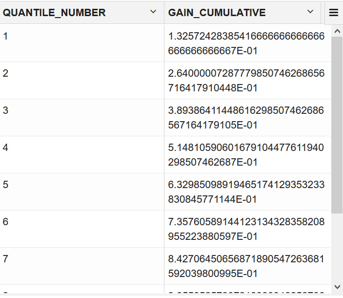
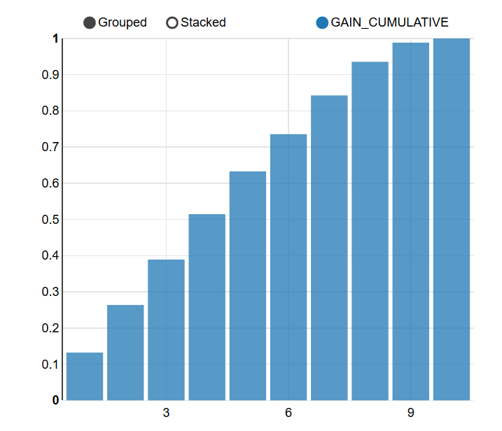
3. To view the cumulative gains, run the following statement:

   Cumulative gain is the ratio of the cumulative number of positive targets (HOME_THEATER_PACKAGE) to the total number of positive targets of a quantile. Cumulative gains act as a visual aid for measuring performance of a model. The chart consists of a curve and a baseline. The greater the area between the curve and the baseline, the better the model.

   %sql
   SELECT QUANTILE_NUMBER, GAIN_CUMULATIVE FROM LIFT_TABLE;

   
4. To compute confusion matrix, run the following statement:
   A confusion matrix evaluates the prediction results. It makes it easy to understand and estimate the effects of wrong predictions. You can observe the number and percentages in each cell of this matrix and notice how often the model predicted accurately.

   %script
   
   DECLARE
      v_accuracy NUMBER;       
      BEGIN
           DBMS_DATA_MINING.COMPUTE_CONFUSION_MATRIX (
                      accuracy => v_accuracy,
                      apply_result_table_name => 'apply_result',
                      target_table_name => 'test_data',
                      case_id_column_name => 'cust_id',
                      target_column_name => 'HOME_THEATER_PACKAGE',
                      confusion_matrix_table_name => 'confusion_matrix',
                      score_column_name => 'PREDICTION',
                      score_criterion_column_name => 'PROBABILITY',
                      cost_matrix_table_name => null,
                      apply_result_schema_name => null,
                      target_schema_name => null,
                      cost_matrix_schema_name => null,
                      score_criterion_type => 'PROBABILITY');
           DBMS_OUTPUT.PUT_LINE('**** MODEL ACCURACY ****: ' || ROUND(v_accuracy,4));
         END;
         /

   **** MODEL ACCURACY ****: .696
   ---------------------------
   PL/SQL procedure successfully completed.
   ---------------------------
   

   Examine the script:

   v_accuracy is a variable declared for this procedure to store and output the model accuracy percentage.

   The COMPUTE_CONFUSION_MATRIX procedure has the following parameters:

   • accuracy: Output parameter containing the overall percentage accuracy of the predictions. Here, it is v_accuracy.
   • apply_result_table_name: Table containing the predictions. In this use case, it is APPLY_RESULT.
   • target_table_name: Table containing the known target values from the test data. In this use case, you are using TEST_DATA.
   • case_id_column_name: Case ID column in the apply results table. Must match the case identifier in the targets table. Here, it is CUST_ID.
   • target_column_name: Target column in the targets table. Contains the known target values from the test data. In this use case, the target column is HOME_THEATER_PACKAGE.
   • confusion_matrix_table_name: Table containing the confusion matrix. The table will be created by the procedure in the user's schema. Here set it as confusion_matrix.
   • score_column_name: Column containing the predictions in the apply results table. The default column name is PREDICTION, which is the default name created by the APPLY procedure.
   • score_criterion_column_name: Column containing the scoring criterion in the apply results table. Contains either the probabilities or the costs that determine the predictions. By default, scoring is based on probability; the class with the highest probability is predicted for each case. If scoring is based on cost, the class with the lowest cost is predicted. The score_criterion_type parameter indicates whether probabilities or costs will be used for scoring. The default column name is 'PROBABILITY', which is the default name created by the APPLY procedure.
   • cost_matrix_table_name: (Optional) Table that defines the costs associated with misclassifications. If a cost matrix table is provided and the score_criterion_type parameter is set to 'COSTS', the costs in this table will be used as the scoring criteria. Otherwise, set it as null.
   • apply_result_schema_name: Schema of the apply results table. If null, the user's schema is assumed.
   • target_schema_name: Schema of the table containing the known targets. If null, the user's schema is assumed.
   • cost_matrix_schema_name: Schema of the cost matrix table, if one is provided. If null, the user's schema is assumed.
   • score_criterion_type: Whether to use probabilities or costs as the scoring criterion. Probabilities or costs are passed in the column identified in the score_criterion_column_name parameter. The default value of score_criterion_type is 'PROBABILITY'. To use costs as the scoring criterion, specify 'COST'. If score_criterion_type is set to 'COST' but no cost matrix is provided and if there is a scoring cost matrix associated with the model, then the associated costs are used for scoring.

   DBMS_OUTPUT.PUT_LINE('**** MODEL ACCURACY ****: ' || ROUND(v_accuracy,4)): Outputs the model accuracy percentage rounded to 4 digits after the decimal.

5. To check the confusion matrix with predicted values and actual values, run the following statement:

   select * from confusion_matrix;

   
   ACTUAL_TARGET_VALUE   PREDICTED_TARGET_VALUE   VALUE   
                       0                        1     501 
                       0                        0     282 
                       1                        0      38 
                       1                        1     952 
   
   ---------------------------

   The value column here indicates classification. From this confusion matrix, the model has predicted actual positive class (also called as True Positive (TP)) for this use case 952 times and incorrectly predicted (also called as False Negative (FN)) for this use case 38 times. The model correctly predicted the negative class (also called true negative (TN)) for this use case 282 times and incorrectly predicted (also called false positive (FP)) for this use case 501 times.

The accuracy percentage of 69% shows that the model is fairly good for this use case.

Score

You are ready to predict the likely customers for the HOME_THEATER_PACKAGE responders. For classification problems, you can use PREDICTION, PREDICTION_PROBABILITY, or use analytic syntax to arrive at predictions.

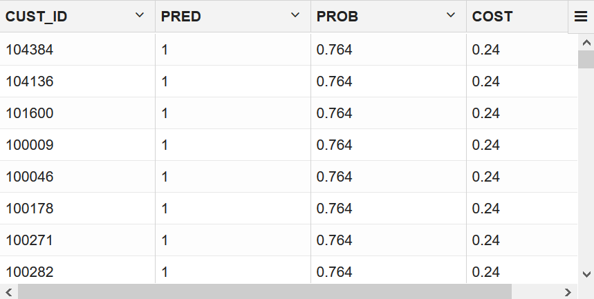
1. To view customers who have more than 50% chance of buying a home theater package, run the following statement:

   %sql
   SELECT CUST_ID, PREDICTION PRED, ROUND(PROBABILITY,3) PROB, ROUND(COST,2) COST
     FROM APPLY_RESULT WHERE PREDICTION = 1 AND PROBABILITY > 0.5
     ORDER BY PROBABILITY DESC;

   
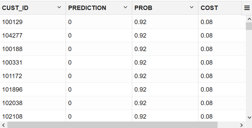
2. You can score on multiple rows of test data. This is called batch scoring. This step shows how you can view and select customers who are likely or unlikely to respond to HOME_THEATER_PACKAGE with a probability of more than 50% and a cost matrix.

   %sql
    
   SELECT CUST_ID, PREDICTION, ROUND(PROBABILITY,2) PROB, ROUND(COST,2) COST
     FROM APPLY_RESULT WHERE PREDICTION = ${PREDICTION='1','1'|'0'}
     AND PROBABILITY > 0.5 ORDER BY PROBABILITY DESC;

   
3. To interactively view probability of HOME_THEATER_PACKAGE respondents, run the following statement:

   %sql
   SELECT A.*, B.*
     FROM APPLY_RESULT A, TEST_DATA B
     WHERE PREDICTION = ${PREDICTION='1','1'|'0'} AND A.CUST_ID = B.CUST_ID;

   
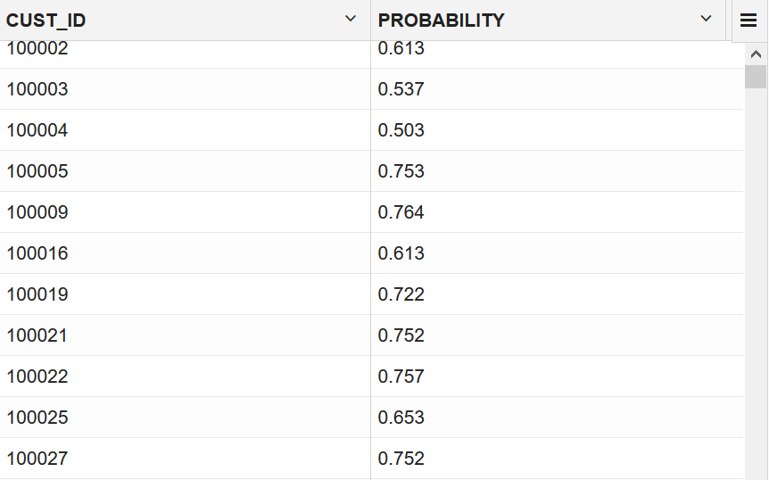
4. To dynamically score and select customers with more than 50% chance of purchasing a home theater package, run the following statement:

   %sql
    
   SELECT *
   FROM (  SELECT CUST_ID, ROUND(PREDICTION_PROBABILITY(MODEL_RF, '1'  USING A.*),3) PROBABILITY
       FROM TEST_DATA A)
   WHERE PROBABILITY > 0.5;
   

   You can use PREDICTION_PROBABILITY to score in real-time.
   
5. To apply the model to a single record (singleton scoring), run the following statement:

   %script
   SELECT ROUND(PREDICTION_PROBABILITY(MODEL_RF, '1' USING
                                       '3' AS HOUSEHOLD_SIZE,
                                        5 AS YRS_RESIDENCE,
                                        1 AS CUST_INCOME_LEVEL),3) PROBABILITY_HOME_THEATER_PACKAGE_RESPONDER
     FROM DUAL;

   This may be useful if you want to test the model manually and see how the model works.

   
   PROBABILITY_HOME_TEATER_PACKAGE_RESPONDER   
                                          0.65 
   
   ---------------------------

To conclude, you have successfully identified customers who are likely to purchase HOME_THEATER_PACKAGE. This prediction helps to promote and offer home theater package to the target customers.