Clustering Use Case Scenario

You're a game data scientist. Marketing team wants to promote a new game and want customers who bought a gaming product with a high credit limit. They want to segment customers based on game purchases and credit level. You help them identify target customers and segment the population using k-Means.

Related Content

Topic	Link
OML4SQL GitHub Example	Clustering - k-Means
CREATE_MODEL2 Procedure	CREATE_MODEL2 Procedure
Generic Model Settings	DBMS_DATA_MINING - Model Settings
k-Means Settings	DBMS_DATA_MINING - Algorithm Settings: k-Means
Data Dictionary Settings	Oracle Machine Learning Data Dictionary Views
k-Means - Model Detail Views	Model Detail Views for k-Means
About Clustering	About Clustering
About k-Means	About k-Means

Before you start your OML4SQL use case journey, ensure that you have the following:

• Data Set

  The data set used for this use case is from the SH schema. The SH schema can be readily accessed in Oracle Autonomous Database. For on-premises databases, the schema is installed during the installation or can be manually installed by downloading the scripts. See Installing the Sample Schemas.

• Database
  Select or create database out of the following options:

  • Get your FREE cloud account. Go to https://cloud.oracle.com/database and select Oracle Database Cloud Service (DBCS), or Oracle Autonomous Database. Create an account and create an instance. See Autonomous Database Quick Start Workshop.
  • Download the latest version of Oracle Database (on premises).
• Machine Learning Tools
  Depending on your database selection,

  • Use OML Notebooks for Oracle Autonomous Database.
  • Install and use Oracle SQL Developer connected to an on-premises database or DBCS. See Installing and Getting Started with SQL Developer.
• Other Requirements

  Data Mining Privileges (this is automatically set for ADW). See System Privileges for Oracle Machine Learning for SQL.

Load Data

Access the data set from the SH Schema and explore the data to understand the attributes.

Remember:

The data set used for this use case is from the SH schema. The SH schema can be readily accessed in Oracle Autonomous Database. For on-premises databases, the schema is installed during the installation or can be manually installed by downloading the scripts. See Installing the Sample Schemas.

To understand the data, you will perform the following:

• Access the data.
• Examine the various attributes or columns of the data set.
• Assess data quality (by exploring the data).

Access Data

You will use CUSTOMERS and SUPPLEMENTARY_DEMOGRAPHICS table data from the SH schema.

Examine Data

The following table displays information about the attributes from SUPPLEMENTARY_DEMOGRAPHICS:

Attribute Name	Information
CUST_ID	The ID of the customer
EDUCATION	Educational information of the customer
OCCUPATION	Occupation of the customer
HOUSEHOLD_SIZE	People per house
YRS_RESIDENCE	Number of years of residence
AFFINITY_CARD	Whether the customer holds an affinity card
BULK_PACK_DISKETTES	Product. Indicates whether the customer already owns the product. 1 means Yes. 0 means No
FLAT_PANEL_MONITOR	Product. Indicates whether the customer already owns the product. 1 means Yes. 0 means No
HOME_THEATER_PACKAGE	Product. Indicates whether the customer already owns the product. 1 means Yes. 0 means No
BOOKKEEPING_APPLICATION	Product. Indicates whether the customer already owns the product. 1 means Yes. 0 means No
PRINTER_SUPPLIES	Product. Indicates whether the customer already owns the product. 1 means Yes. 0 means No
Y_BOX_GAMES	Product. Indicates whether the customer already owns the product. 1 means Yes. 0 means No
OS_DOC_SET_KANJI	Product. Indicates whether the customer already owns the product. 1 means Yes. 0 means No
COMMENTS	Product. Indicates whether the customer already owns the product. 1 means Yes. 0 means No

Explore Data

Once the data is accessible, explore the data to understand and assess the quality of the data. At this stage assess the data to identify data types and noise in the data. Look for missing values and numeric outlier values.

Assess Data Quality

To assess the data, first, you must be able to view the data in your database. For this reason, you will use SQL statements to query the SH.CUSTOMERS and the SH.SUPPLEMENTARY_DEMOGRAPHICS table.

If you are working with Oracle Autonomous Database, you can use the Oracle Machine Learning (OML) Notebooks for your data science project, including assessing data quality. If you are using on-premise Oracle Database, you can use the Oracle SQL Developer to assess data quality. Query the SH schema as described.

Note:

Each record in the database is called a case and each case is identified by a case_id. In this use case, CUST_ID is the case_id.

The following steps help you with the exploratory analysis of the data:

1. View the data in the SH.CUSTOMERS table by running the following query:

   SELECT * FROM SH.CUSTOMERS;

2. To see distinct data from the table, run the following query:

   SELECT DISTINCT * FROM SH.CUSTOMERS;

   
3. Find the COUNT rows in the data set, run the following statement:

   SELECT DISTINCT COUNT(*) from SH.CUSTOMERS;

   COUNT(*)   
        55500 
   ---------------------------

4. To find distinct or unique customers in the table, run the following statement:

   %script
   SELECT COUNT (DISTINCT CUST_ID) FROM SH.CUSTOMERS;

   COUNT(DISTINCTCUST_ID)   
                      55500 
   ---------------------------

5. Similarly, query the SH.SUPPLEMENTARY_DEMOGRAPHICS table.

   SELECT * FROM SH.SUPPLEMENTARY_DEMOGRAPHICS;

   
6. To view the count of rows in the SH.SUPPLEMENTARY_DEMOGRAPHICS table, run the following statement:

   SELECT COUNT(*) from SH.SUPPLEMENTARY_DEMOGRAPHICS;
   

   COUNT(*)   
         4500 
   ---------------------------

7. Create a table called CUSTOMERDATA by selecting the required columns from the SH.CUSTOMERS and the SH.SUPPLIMENTARY_DEMOGRAPHICS tables.

   %script
    
   CREATE OR REPLACE VIEW CUSTOMERDATA AS
      SELECT a.CUST_ID, a.CUST_GENDER, a.CUST_MARITAL_STATUS,
             a.CUST_YEAR_OF_BIRTH, a.CUST_INCOME_LEVEL, a.CUST_CREDIT_LIMIT,
             b.HOUSEHOLD_SIZE, b.YRS_RESIDENCE, b.Y_BOX_GAMES
      FROM SH.CUSTOMERS a, SH.SUPPLEMENTARY_DEMOGRAPHICS b
      WHERE a.CUST_ID = b.CUST_ID;
    

   View CUSTOMERDATA created.

8. View the CUSTOMERDATA table.

   SELECT * FROM CUSTOMERDATA;

   
9. Find the count of rows in the new CUSTOMERDATA table:

   SELECT COUNT(*) FROM CUSTOMERDATA;

   COUNT(*)   
         4500 
   ---------------------------

10. To view the data type of the columns, run the following statement:

    %script
    DESCRIBE CUSTOMERDATA;

    
    Name                Null?    Type        
    ------------------- -------- ------------
    CUST_ID       	   NOT NULL  NUMBER
    CUST_GENDER 	   NOT NULL  CHAR(1)
    CUST_MARITAL_STATUS          VARCHAR2(20)
    CUST_YEAR_OF_BIRTH NOT NULL  NUMBER(4)
    CUST_INCOME_LEVEL            VARCHAR2(30)
    CUST_CREDIT_LIMIT            NUMBER
    HOUSEHOLD_SIZE               VARCHAR2(21)
    YRS_RESIDENCE                NUMBER
    Y_BOX_GAMES          	 NUMBER(10)
     
    ---------------------------

11. To check if there are any missing values (NULL values), run the following statement:

    SELECT COUNT(*) FROM CUSTOMERDATA WHERE CUST_ID=NULL OR CUST_GENDER=NULL
     OR CUST_MARITAL_STATUS=NULL OR CUST_YEAR_OF_BIRTH=NULL OR CUST_INCOME_LEVEL=NULL
     OR CUST_CREDIT_LIMIT=NULL OR HOUSEHOLD_SIZE=NULL OR YRS_RESIDENCE=NULL OR Y_BOX_GAMES=NULL;
    
    

    COUNT(*)   
             0 
    ---------------------------

    NULLs, if found, are automatically handled by the OML algorithms. Alternately, you can manually replace NULLs with NVL SQL function.

This completes the data exploration stage. OML supports Automatic Data Preparation (ADP). ADP is enabled through the model settings. When ADP is enabled, the transformations required by the algorithm are performed automatically and embedded in the model. This step is done during the Build Model stage. The commonly used methods of data preparation are binning, normalization, and missing value treatment.

Build Model

Build your model using your data set. Use the DBMS_DATA_MINING.CREATE_MODEL2 procedure to build your model and specify the model settings.

To evaluate the model and to accurately assess the performance of the model on the same data, you generally split or separate the data into training and test data. For an unsupervised learning, like Clustering, you do not have labels or predictors to calculate the accuracy or assess the performance. Thus, you can create a model using your data set without splitting. For an unsupervised learning, you don't have a real way of knowing how good your model is. So, a training or a test split is not useful.

Algorithm Selection

Before you build a model, choose the suitable algorithm. You can choose one of the following algorithms to solve a clustering problem:

• k-Means
• Expectation Maximization (EM)
• Orthogonal Cluster (O-Cluster)

K-Means does not assume a particular distribution of the data. The k-Means algorithm is a distance-based clustering algorithm that partitions the data into a specified number of clusters. The EM algorithm is a probability density estimation technique. EM method is based on assumption that the data has several clusters and each cluster is distributed according to a certain Gaussian distribution. O-Cluster is a neighbor based method. It identifies areas of high density in the data and separates the dense areas into clusters. It is able to cluster data points that forms a certain shape, which sometimes can be a complex pattern like a circle, spiral, or even a tie shape.

K-Means tends to cluster points only close to each other and does not necessarily cluster the data based on the shapes. Therefore, K-Means method is the one with the simplest assumption. Thus, it is the clustering method to start with.

The following steps guide you to build your model with the selected algorithm.

1. Build your model using the CREATE_MODEL2 procedure. First, declare a variable to store model settings or hyperparameters. Run the following script:

   %script
    
   BEGIN DBMS_DATA_MINING.DROP_MODEL('KM_SH_CLUS1');
   EXCEPTION WHEN OTHERS THEN NULL; END;
   /
   DECLARE
       v_setlist DBMS_DATA_MINING.SETTING_LIST;
   BEGIN
       v_setlist('ALGO_NAME')        := 'ALGO_KMEANS';
       V_setlist('PREP_AUTO')        := 'ON';
       V_setlist('KMNS_DISTANCE')    := 'KMNS_EUCLIDEAN';
       V_setlist('KMNS_DETAILS')     := 'KMNS_DETAILS_ALL';
       V_setlist('KMNS_ITERATIONS')  := '10';
       V_setlist('KMNS_NUM_BINS')    := '10';
       v_setlist('CLUS_NUM_CLUSTERS'):= '1';
    
       DBMS_DATA_MINING.CREATE_MODEL2(
           MODEL_NAME          => 'KM_SH_CLUS1',
           MINING_FUNCTION     => 'CLUSTERING',
           DATA_QUERY          => 'select * from CUSTOMERDATA',
           SET_LIST            => v_setlist,
           CASE_ID_COLUMN_NAME => 'CUST_ID');
   END;
    
   

   
   PL/SQL procedure successfully completed.
   ---------------------------
   PL/SQL procedure successfully completed.
   

   Examine the script:

   • v_setlist is a variable to store SETTING_LIST.
   • SETTING_LIST specifies model settings or hyperparameters for our model.
   • DBMS_DATA_MINING is the PL/SQL package used for machine learning. These settings are described in DBMS_DATA_MINING - Model Settings.
   • ALGO_NAME specifies the algorithm name. Since you are using the k-Means as your algorithm, set ALGO_KMEANS.
   • PREP_AUTO is the setting used for Automatic Data Preparation. Here, enable Automatic Data Preparation. The value of the setting is ON.
   • KMNS_DISTANCE is the distance function that measures the similarity between the cases for k-Means. The value here is KMNS_EUCLIDEAN. This is the default value.
   • KMNS_DETAILS determines the level of cluster details. KMNS_DETAILS_ALL computes cluster hierarchy, record counts, descriptive statistics (means, variances, modes, histograms, and rules).
   • KMNS_ITERATIONS defines the maximum number of iterations for k-Means. The algorithm iterates until either the maximum number of iterations are reached or the minimum Convergence Tolerance, specified in KMNS_CONV_TOLERANCE, is satisfied. The default number of iterations is 20.
   • KMNS_NUM_BINS provides a number of bins in the attribute histogram produced by k-Means.
   • CLUS_NUM_CLUSTERS is the maximum number of leaf clusters generated by a clustering algorithm. The algorithm may return fewer clusters, depending on the data. Enhanced k-Means usually produces the exact number of clusters specified by CLUS_NUM_CLUSTERS, unless there are fewer distinct data points.

   The CREATE_MODEL2 procedure takes the following parameters:

   • MODEL_NAME: A unique model name that you will give to your model. The name of the model is in the form [schema_name.]model_name. If you do not specify a schema, then your own schema is used. Here, the model name is KM_SH_CLUS1.
   • MINING_FUNCTION: Specifies the machine learning function. Since you are solving a clustering problem in this use case, select CLUSTERING.
   • DATA_QUERY: A query that provides training data for building the model. Here, the query is SELECT * FROM CUSTOMERDATA.
   • SET_LIST: Specifies SETTING_LIST.
   • CASE_ID_COLUMN_NAME: A unique case identifier column in the build data. In this use case, case_id is CUST_ID. If there is a composite key, you must create a new attribute before creating the model. This may involve concatenating values from the columns, or mapping a unique identifier to each distinct combination of values. The CASE_ID assists with reproducible results, joining scores for individual customers with other data in, example, scoring data table.

   Note:

   Any parameters or settings not specified are either system-determined or default values are used.

Evaluate

Evaluate your model by viewing diagnostic metrics and performing quality checks.

Sometimes querying dictionary views and model detail views is sufficient to measure your model's performance. However, you can evaluate your model by computing test metrics such as Mean Absolute Error (MAE), Root Mean Squared Error (RMSE), confusion matrix, lift statistics, cost matrix, and so on. For Association Rules, you can inspect various rules to see if they reveal new insights for item dependencies (antecedent itemset implying consequent) or for unexpected relationships among items.

Dictionary and Model Views

To obtain information about the model and view model settings, you can query data dictionary views and model detail views. Specific views in model detail views display model statistics which can help you evaluate the model.

The data dictionary views for Oracle Machine Learning are listed in the following table. A database administrator (DBA) and USER versions of the views are also available.

View Name	Description
ALL_MINING_MODELS	Provides information about all accessible machine learning models
ALL_MINING_MODEL_ATTRIBUTES	Provides information about the attributes of all accessible machine learning models
ALL_MINING_MODEL_SETTINGS	Provides information about the configuration settings for all accessible machine learning models
ALL_MINING_MODEL_VIEWS	Provides information about the model views for all accessible machine learning models
ALL_MINING_MODEL_XFORMS	Provides the user-specified transformations embedded in all accessible machine learning models.

Model detail views are specific to the algorithm. You can obtain more insights about the model you created by viewing the model detail views. The names of model detail views begin with DM$xx where xx corresponds to the view prefix. See Model Detail Views.

The following steps help you to view different dictionary views and model detail views.

1. Run the following statement to view the settings in USER_MINING_MODEL_SETTINGS:

   %script
   SELECT SETTING_NAME, SETTING_VALUE
   FROM USER_MINING_MODEL_SETTINGS
   WHERE MODEL_NAME = 'KM_SH_CLUS1'
   ORDER BY SETTING_NAME;

   SETTING_NAME                   SETTING_VALUE             
   ALGO_NAME                      ALGO_KMEANS               
   CLUS_NUM_CLUSTERS              1                         
   KMNS_CONV_TOLERANCE            .001                      
   KMNS_DETAILS                   KMNS_DETAILS_ALL          
   KMNS_DISTANCE                  KMNS_EUCLIDEAN            
   KMNS_ITERATIONS                3                         
   KMNS_MIN_PCT_ATTR_SUPPORT      .1                        
   KMNS_NUM_BINS                  10                        
   KMNS_RANDOM_SEED               0                         
   KMNS_SPLIT_CRITERION           KMNS_VARIANCE             
   ODMS_DETAILS                   ODMS_ENABLE               
   ODMS_MISSING_VALUE_TREATMENT   ODMS_MISSING_VALUE_AUTO   
   ODMS_SAMPLING                  ODMS_SAMPLING_DISABLE     
   PREP_AUTO                      ON                        
   
   
   
   14 rows selected. 
   
   
   ---------------------------
   

2. Run the following statement to see attribute information in USER_MINING_MODEL_ATTRIBUTES view:

   %script
   SELECT ATTRIBUTE_NAME, ATTRIBUTE_TYPE
   FROM USER_MINING_MODEL_ATTRIBUTES
   WHERE MODEL_NAME = 'KM_SH_CLUS1'
   ORDER BY ATTRIBUTE_NAME;

   
   ATTRIBUTE_NAME        ATTRIBUTE_TYPE   
   CUST_CREDIT_LIMIT     NUMERICAL        
   CUST_GENDER           CATEGORICAL      
   CUST_INCOME_LEVEL     CATEGORICAL      
   CUST_MARITAL_STATUS   CATEGORICAL      
   CUST_YEAR_OF_BIRTH    NUMERICAL        
   HOUSEHOLD_SIZE        CATEGORICAL      
   YRS_RESIDENCE         NUMERICAL        
   Y_BOX_GAMES           NUMERICAL        
   
   
   8 rows selected. 
   ---------------------------

3. Run the following statement to see information on various views in USER_MINING_MODEL_VIEWS:

   %script
   SELECT VIEW_NAME, VIEW_TYPE FROM USER_MINING_MODEL_VIEWS
   WHERE MODEL_NAME='KM_SH_CLUS1'
   ORDER BY VIEW_NAME;

   
   VIEW_NAME          VIEW_TYPE                                  
   DM$VAKM_SH_CLUS1   Clustering Attribute Statistics            
   DM$VCKM_SH_CLUS1   k-Means Scoring Centroids                  
   DM$VDKM_SH_CLUS1   Clustering Description                     
   DM$VGKM_SH_CLUS1   Global Name-Value Pairs                    
   DM$VHKM_SH_CLUS1   Clustering Histograms                      
   DM$VNKM_SH_CLUS1   Normalization and Missing Value Handling   
   DM$VRKM_SH_CLUS1   Clustering Rules                           
   DM$VSKM_SH_CLUS1   Computed Settings                          
   DM$VWKM_SH_CLUS1   Model Build Alerts                         
   
   
   9 rows selected. 
   
   
   ---------------------------

4. Now, view the Clustering Description model detail view:

   SELECT CLUSTER_ID CLU_ID, RECORD_COUNT REC_CNT, PARENT,
          TREE_LEVEL, ROUND(TO_NUMBER(DISPERSION),3) DISPERSION
   FROM   DM$VDKM_SH_CLUS1
   ORDER BY CLUSTER_ID;

   
   CLU_ID   REC_CNT   PARENT   TREE_LEVEL   DISPERSION   
          1      4500                     1        6.731 
   
   ---------------------------

5. To see the leaf cluster IDs, run the following query:

   Oracle supports hierarchical clustering. In hierarchical clustering, the data points having similar characteristics are grouped together. The cluster hierarchy is represented as a tree structure. The leaf clusters are the final clusters generated by the algorithm. Clusters higher up in the hierarchy are intermediate clusters.

   SELECT CLUSTER_ID
   FROM   DM$VDKM_SH_CLUS1
   WHERE LEFT_CHILD_ID IS NULL AND RIGHT_CHILD_ID IS NULL
   ORDER BY CLUSTER_ID;

   
   CLUSTER_ID   
              1 
   ---------------------------

   Examine the query:

   LEFT_CHILD_ID IS NULL: Outputs the leaf nodes on the left of the hierarchical tree

   RIGHT_CHILD_ID IS NULL: Outputs the leaf nodes on the right of the hierarchical tree

6. View the dispersion details or the cluster description for the leaf cluster IDs:
   Dispersion is a measure of cluster quality and computationally it is the sum of squared error. This also indicates the quality of the cluster model.

   %script
   SELECT CLUSTER_ID CLU_ID, RECORD_COUNT REC_CNT, PARENT, 
          TREE_LEVEL, ROUND(TO_NUMBER(DISPERSION),3) DISPERSION
   FROM   DM$VDKM_SH_CLUS1
   WHERE CLUSTER_ID IN (SELECT CLUSTER_ID
                        FROM   DM$VDKM_SH_CLUS1
                        WHERE LEFT_CHILD_ID IS NULL AND RIGHT_CHILD_ID IS NULL)
   ORDER BY CLUSTER_ID;

   
   CLU_ID   REC_CNT   PARENT   TREE_LEVEL   DISPERSION   
          1      4500                     1        6.731 
   
   ---------------------------

7. To determine the optimal value of K (or the number of clusters) for the data, visualize the data with an Elbow method.
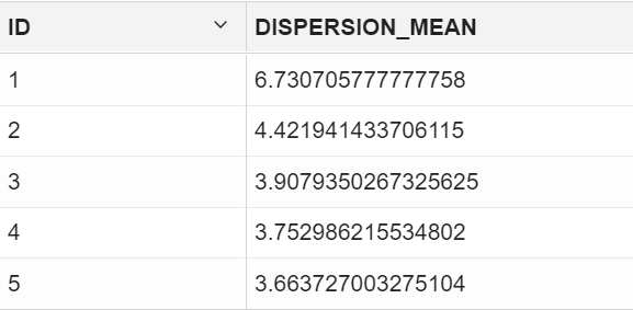
   The Elbow method is done with the leaf clusters. In cluster analysis, the elbow method is a heuristic used in determining the number of clusters in a data set. The method consists of plotting the variance (or dispersion) as a function of the number of clusters and picking the elbow of the curve as the number of clusters to use.

   %sql
   SELECT 1 ID, AVG(DISPERSION) DISPERSION_MEAN
   FROM   DM$VDKM_SH_CLUS1 
   WHERE LEFT_CHILD_ID IS NULL AND RIGHT_CHILD_ID IS NULL
   UNION
   SELECT 2 ID, AVG(DISPERSION) DISPERSION_MEAN
   FROM   DM$VDKM_SH_CLUS2
   WHERE LEFT_CHILD_ID IS NULL AND RIGHT_CHILD_ID IS NULL
   UNION
   SELECT 3 ID, AVG(DISPERSION) DISPERSION_MEAN
   FROM   DM$VDKM_SH_CLUS3
   WHERE LEFT_CHILD_ID IS NULL AND RIGHT_CHILD_ID IS NULL
   UNION
   SELECT 4 ID, AVG(DISPERSION) DISPERSION_MEAN
   FROM   DM$VDKM_SH_CLUS4
   WHERE LEFT_CHILD_ID IS NULL AND RIGHT_CHILD_ID IS NULL
   UNION
   SELECT 5 ID, AVG(DISPERSION) DISPERSION_MEAN
   FROM   DM$VDKM_SH_CLUS5
   WHERE LEFT_CHILD_ID IS NULL AND RIGHT_CHILD_ID IS NULL;

   

   From the resultant graph, the curve flattens after 3 or the dispersion value flattens after ID 3, which means that the optimal value of K (or the most suitable number of clusters that the data must be segmented into) is 3.

   Note:

   In Oracle SQL Developer, a visual aid to view the graph is not applicable. You can only compute the dispersion scores.
8. To view the Attribute details of the KM_SH_CLUS3 model, run the following statement:
   The Attribute Details view displays statistics like mean, median, and mode of your model.

   %script
   SELECT CLUSTER_ID, ATTRIBUTE_NAME, ATTRIBUTE_SUBNAME, MEAN, VARIANCE, MODE_VALUE
   FROM  DM$VAKM_SH_CLUS3;

   
   CLUSTER_ID   ATTRIBUTE_NAME        ATTRIBUTE_SUBNAME   MEAN                  VARIANCE             MODE_VALUE             
              1 CUST_CREDIT_LIMIT                         7924.222222222223     15914238.670321768                          
              1 CUST_YEAR_OF_BIRTH                        1964.6244444444444    187.1267639722414                           
              1 YRS_RESIDENCE                             4.021999999999995     3.617430984663253                           
              1 Y_BOX_GAMES                               0.31244444444444447   0.2148706626163839                          
              1 CUST_GENDER                                                                          M                      
              1 CUST_INCOME_LEVEL                                                                    J: 190,000 - 249,999   
              1 CUST_MARITAL_STATUS                                                                  Married                
              1 HOUSEHOLD_SIZE                                                                       3                      
              2 CUST_CREDIT_LIMIT                         7833.002645502645     15543554.858080933                          
              2 CUST_YEAR_OF_BIRTH                        1957.631283068783     121.54941469457282                          
              2 YRS_RESIDENCE                             4.8611111111111045    2.7838791487484835                          
              2 Y_BOX_GAMES                               0.0                   0.0                                         
              2 CUST_GENDER                                                                          M                      
              2 CUST_INCOME_LEVEL                                                                    J: 190,000 - 249,999   
   
   CLUSTER_ID   ATTRIBUTE_NAME        ATTRIBUTE_SUBNAME   MEAN                 VARIANCE              MODE_VALUE             
              2 CUST_MARITAL_STATUS                                                                  Married                
              2 HOUSEHOLD_SIZE                                                                       3                      
              3 CUST_CREDIT_LIMIT                         8111.111111111114    16632730.696798513                           
              3 CUST_YEAR_OF_BIRTH                        1978.9518970189702   15.976667585319932                           
              3 YRS_RESIDENCE                             2.3028455284552827   0.9272054568003305                           
              3 Y_BOX_GAMES                               0.9525745257452575   0.04520692664553768                          
              3 CUST_GENDER                                                                          M                      
              3 CUST_INCOME_LEVEL                                                                    J: 190,000 - 249,999   
              3 CUST_MARITAL_STATUS                                                                  NeverM                 
              3 HOUSEHOLD_SIZE                                                                       1                      
              4 CUST_CREDIT_LIMIT                         3126.6094420600857   2978559.2320826976                           
              4 CUST_YEAR_OF_BIRTH                        1978.4978540772531   22.143006137800537                           
              4 YRS_RESIDENCE                             2.270386266094421    0.8944759795099003                           
              4 Y_BOX_GAMES                               0.8819742489270386   0.10431953481932726                          
   
   CLUSTER_ID   ATTRIBUTE_NAME        ATTRIBUTE_SUBNAME   MEAN                 VARIANCE              MODE_VALUE             
              4 CUST_GENDER                                                                          F                      
              4 CUST_INCOME_LEVEL                                                                    B: 30,000 - 49,999     
              4 CUST_MARITAL_STATUS                                                                  NeverM                 
              4 HOUSEHOLD_SIZE                                                                       1                      
              5 CUST_CREDIT_LIMIT                         10410.891089108914   6172923.883072166                            
              5 CUST_YEAR_OF_BIRTH                        1979.1613861386138   13.01158975164117                            
              5 YRS_RESIDENCE                             2.3178217821782146   0.9424967372852242                           
              5 Y_BOX_GAMES                               0.9851485148514851   0.01464541895220246                          
              5 CUST_GENDER                                                                          M                      
              5 CUST_INCOME_LEVEL                                                                    J: 190,000 - 249,999   
              5 CUST_MARITAL_STATUS                                                                  NeverM                 
              5 HOUSEHOLD_SIZE                                                                       1                      
   
   
   40 rows selected.

   Notice that Cluster ID 5 has the highest mean for Y_BOX_GAMES users and has the highest CUST_CREDIT_LIMIT.

9. Now, for the model KM_SH_CLUS3, view the histogram details with specific attributes for each leaf cluster. For this use-case, view the histogram details for Y_BOX_GAMES and CUST_INCOME_LEVEL attributes. In this step, leaf cluster ID 5 and the attribute Y_BOX_GAMES are picked.

   %sql
    
   SELECT CLUSTER_ID, ATTRIBUTE_NAME, ATTRIBUTE_SUBNAME,
          BIN_ID, LOWER_BIN_BOUNDARY, UPPER_BIN_BOUNDARY, ATTRIBUTE_VALUE, COUNT
   FROM DM$VHKM_SH_CLUS3
   WHERE CLUSTER_ID = 5 AND ATTRIBUTE_NAME = 'Y_BOX_GAMES'
   ORDER BY BIN_ID;

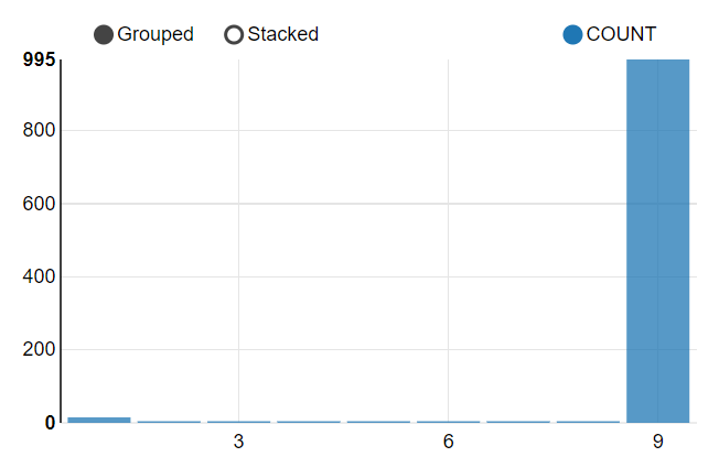
   In OML Notebooks, click the bar plot icon and expand settings. Drag BIN_ID to keys and COUNT to values.
   

   From this histogram, you can see that Cluster ID 5 is grouped into bins showing the count of Y_BOX_GAMES users. Bin 9 has the highest count of Y_BOX_GAMES users.

10. Similarly, for Cluster ID 5, view the histogram details for the CUST_INCOME_LEVEL attribute.

    %sql
     
    SELECT CLUSTER_ID, ATTRIBUTE_NAME, ATTRIBUTE_SUBNAME,
           BIN_ID, LOWER_BIN_BOUNDARY, UPPER_BIN_BOUNDARY, ATTRIBUTE_VALUE, COUNT
    FROM DM$VHKM_SH_CLUS3
    WHERE CLUSTER_ID = 5 AND ATTRIBUTE_NAME = 'CUST_INCOME_LEVEL'
    ORDER BY BIN_ID;

    In OML Notebooks, click the bar plot icon and expand settings. Drag BIN_ID and ATTRIBUTE_VALUE to keys and COUNT to values. In the xAxis options, click Rotate.
    

    In this histogram, Cluster ID 5 is grouped into bins showing the count of customers with CUST_INCOME_LEVEL and indicates that the highest number of customers draw a salary package between 190,000 - 249,999 yearly.

11. Now, view the Rule details of leaf clusters (2, 4, and 5) to check the support and confidence level.
    Support and confidence are metrics that describe the relationships between clustering rules and cases. Support is the percentage of cases for which the rule holds. Confidence is the probability that a case described by this rule is actually assigned to the cluster.

    %script
     
    SELECT CLUSTER_ID, ATTRIBUTE_NAME, ATTRIBUTE_SUBNAME, OPERATOR,
           NUMERIC_VALUE, ATTRIBUTE_VALUE, SUPPORT, ROUND(CONFIDENCE,3) CONFIDENCE
    FROM DM$VRKM_SH_CLUS3
    WHERE cluster_id IN (SELECT cluster_id
                         FROM DM$VDKM_SH_CLUS3
                         WHERE LEFT_CHILD_ID is NULL and RIGHT_CHILD_ID is NULL)
    ORDER BY CLUSTER_ID, ATTRIBUTE_NAME, ATTRIBUTE_SUBNAME, OPERATOR, NUMERIC_VALUE, ATTRIBUTE_VALUE;

    
    CLUSTER_ID   ATTRIBUTE_NAME        ATTRIBUTE_SUBNAME   OPERATOR   NUMERIC_VALUE   ATTRIBUTE_VALUE        SUPPORT   CONFIDENCE   
               2 CUST_CREDIT_LIMIT                         <=         15000.0                                     3024            0 
               2 CUST_CREDIT_LIMIT                         >=         1500.0                                      3024            0 
               2 CUST_GENDER                               IN                         F                           3024        0.002 
               2 CUST_GENDER                               IN                         M                           3024        0.002 
               2 CUST_INCOME_LEVEL                         IN                         B: 30,000 - 49,999          2750            0 
               2 CUST_INCOME_LEVEL                         IN                         E: 90,000 - 109,999         2750            0 
               2 CUST_INCOME_LEVEL                         IN                         F: 110,000 - 129,999        2750            0 
               2 CUST_INCOME_LEVEL                         IN                         G: 130,000 - 149,999        2750            0 
               2 CUST_INCOME_LEVEL                         IN                         H: 150,000 - 169,999        2750            0 
               2 CUST_INCOME_LEVEL                         IN                         I: 170,000 - 189,999        2750            0 
               2 CUST_INCOME_LEVEL                         IN                         J: 190,000 - 249,999        2750            0 
               2 CUST_INCOME_LEVEL                         IN                         K: 250,000 - 299,999        2750            0 
               2 CUST_INCOME_LEVEL                         IN                         L: 300,000 and above        2750            0 
               2 CUST_MARITAL_STATUS                       IN                         Divorc.                     2720        0.014 
    
    CLUSTER_ID   ATTRIBUTE_NAME        ATTRIBUTE_SUBNAME   OPERATOR   NUMERIC_VALUE        ATTRIBUTE_VALUE   SUPPORT   CONFIDENCE   
               2 CUST_MARITAL_STATUS                       IN                              Married                2720        0.014 
               2 CUST_MARITAL_STATUS                       IN                              NeverM                 2720        0.014 
               2 CUST_YEAR_OF_BIRTH                        <=         1977.888888888889                           2854        0.041 
               2 CUST_YEAR_OF_BIRTH                        >          1937.3333333333333                          2854        0.041 
               2 HOUSEHOLD_SIZE                            IN                              2                      2699        0.016 
               2 HOUSEHOLD_SIZE                            IN                              3                      2699        0.016 
               2 HOUSEHOLD_SIZE                            IN                              9+                     2699        0.016 
               2 YRS_RESIDENCE                             <=         7.777777777777778                           2804        0.019 
               2 YRS_RESIDENCE                             >          1.5555555555555556                          2804        0.019 
               2 Y_BOX_GAMES                               <=         0.1111111111111111                          3024        0.056 
               2 Y_BOX_GAMES                               >=         0.0                                         3024        0.056 
               4 CUST_CREDIT_LIMIT                         <=         7500.0                                       466        0.128 
               4 CUST_CREDIT_LIMIT                         >=         1500.0                                       466        0.128 
               4 CUST_GENDER                               IN                              F                       466        0.023 
    
    CLUSTER_ID   ATTRIBUTE_NAME        ATTRIBUTE_SUBNAME   OPERATOR   NUMERIC_VALUE        ATTRIBUTE_VALUE        SUPPORT   CONFIDENCE   
               4 CUST_GENDER                               IN                              M                            466        0.023 
               4 CUST_INCOME_LEVEL                         IN                              A: Below 30,000              466        0.079 
               4 CUST_INCOME_LEVEL                         IN                              B: 30,000 - 49,999           466        0.079 
               4 CUST_INCOME_LEVEL                         IN                              C: 50,000 - 69,999           466        0.079 
               4 CUST_INCOME_LEVEL                         IN                              D: 70,000 - 89,999           466        0.079 
               4 CUST_INCOME_LEVEL                         IN                              E: 90,000 - 109,999          466        0.079 
               4 CUST_INCOME_LEVEL                         IN                              F: 110,000 - 129,999         466        0.079 
               4 CUST_INCOME_LEVEL                         IN                              G: 130,000 - 149,999         466        0.079 
               4 CUST_INCOME_LEVEL                         IN                              H: 150,000 - 169,999         466        0.079 
               4 CUST_INCOME_LEVEL                         IN                              I: 170,000 - 189,999         466        0.079 
               4 CUST_MARITAL_STATUS                       IN                              Married                      413        0.043 
               4 CUST_MARITAL_STATUS                       IN                              NeverM                       413        0.043 
               4 CUST_YEAR_OF_BIRTH                        <=         1986.0                                            451        0.103 
               4 CUST_YEAR_OF_BIRTH                        >          1969.7777777777778                                451        0.103 
    
    CLUSTER_ID   ATTRIBUTE_NAME      ATTRIBUTE_SUBNAME   OPERATOR   NUMERIC_VALUE       ATTRIBUTE_VALUE        SUPPORT   CONFIDENCE   
               4 HOUSEHOLD_SIZE                          IN                             1                            418        0.043 
               4 HOUSEHOLD_SIZE                          IN                             2                            418        0.043 
               4 HOUSEHOLD_SIZE                          IN                             3                            418        0.043 
               4 HOUSEHOLD_SIZE                          IN                             9+                           418        0.043 
               4 YRS_RESIDENCE                           <=         4.666666666666667                                464        0.086 
               4 YRS_RESIDENCE                           >=         0.0                                              464        0.086 
               4 Y_BOX_GAMES                             <=         1.0                                              466        0.083 
               4 Y_BOX_GAMES                             >=         0.0                                              466        0.083 
               5 CUST_CREDIT_LIMIT                       <=         15000.0                                         1010        0.056 
               5 CUST_CREDIT_LIMIT                       >          6000.0                                          1010        0.056 
               5 CUST_GENDER                             IN                             F                           1010        0.002 
               5 CUST_GENDER                             IN                             M                           1010        0.002 
               5 CUST_INCOME_LEVEL                       IN                             F: 110,000 - 129,999         906        0.024 
               5 CUST_INCOME_LEVEL                       IN                             G: 130,000 - 149,999         906        0.024 
    
    CLUSTER_ID   ATTRIBUTE_NAME        ATTRIBUTE_SUBNAME   OPERATOR   NUMERIC_VALUE        ATTRIBUTE_VALUE        SUPPORT   CONFIDENCE   
               5 CUST_INCOME_LEVEL                         IN                              I: 170,000 - 189,999         906        0.024 
               5 CUST_INCOME_LEVEL                         IN                              J: 190,000 - 249,999         906        0.024 
               5 CUST_INCOME_LEVEL                         IN                              K: 250,000 - 299,999         906        0.024 
               5 CUST_INCOME_LEVEL                         IN                              L: 300,000 and above         906        0.024 
               5 CUST_MARITAL_STATUS                       IN                              Married                      944        0.046 
               5 CUST_MARITAL_STATUS                       IN                              NeverM                       944        0.046 
               5 CUST_YEAR_OF_BIRTH                        <=         1986.0                                           1003         0.12 
               5 CUST_YEAR_OF_BIRTH                        >          1969.7777777777778                               1003         0.12 
               5 HOUSEHOLD_SIZE                            IN                              1                            859        0.036 
               5 HOUSEHOLD_SIZE                            IN                              2                            859        0.036 
               5 HOUSEHOLD_SIZE                            IN                              3                            859        0.036 
               5 YRS_RESIDENCE                             <=         4.666666666666667                                 993        0.079 
               5 YRS_RESIDENCE                             >=         0.0                                               993        0.079 
               5 Y_BOX_GAMES                               <=         1.0                                               995        0.136 
    
    CLUSTER_ID   ATTRIBUTE_NAME   ATTRIBUTE_SUBNAME   OPERATOR   NUMERIC_VALUE        ATTRIBUTE_VALUE   SUPPORT   CONFIDENCE   
               5 Y_BOX_GAMES                          >          0.8888888888888888                           995        0.136 
    
    
    71 rows selected. 
    
    ---------------------------

12. To view the size of each cluster, run the following statement:

    In OML Notebooks, you can also click the bar icon or the pie chart icon to view the bar graph or the pie chart.

    %sql
    SELECT CLUSTER_ID(KM_SH_CLUS3 USING *) AS CLUS, COUNT(*) AS CNT
    FROM CUSTOMERDATA
    GROUP BY CLUSTER_ID(KM_SH_CLUS3 USING *)
    ORDER BY CNT DESC;

    
    CLUS   CNT    
         2   3024 
         5   1010 
         4    466 
    ---------------------------

Score

Scoring involves applying the model to the target data. Use CLUSTER_PROBABILITY function to predict the clusters. For Clustering, "scoring" involves assigning each record to a cluster, with a certain probability. However, one can also obtain the probability of a record belonging to each cluster.

1. In the following step, you are scoring the probability of the top 10 customers that belong to cluster 5.

   %script
    
   SELECT CUST_ID,
          ROUND(CLUSTER_PROBABILITY(KM_SH_CLUS3, 5 USING *),3)
          PROB
   FROM CUSTOMERDATA
   WHERE rownum < 10
   ORDER BY PROB DESC;

   
   CUST_ID   PROB    
      102308   0.539 
      101232   0.502 
      101610   0.374 
      102828   0.303 
      100134   0.302 
      103948   0.297 
      100696    0.25 
      103791   0.141 
      100804   0.104 
   
   
   9 rows selected. 
   
   ---------------------------

2. To score the cluster ID of a given CUST_ID (customer), for this use case, you must target customers who have already purchased Y_BOX_GAMES and with high credit limit, to sell the new game product. In the previous stage, you have identified that cluster 5 has highest customers who have already purchased Y_BOX_GAMES with mean CUST_CREDIT_LIMIT of 10410. So, the target group is cluster ID 5. To score for a given CUST_ID (102308) and display the probability score, run the following query :

   %sql
   SELECT CLUSTER_ID(KM_SH_CLUS3 USING *) AS CLUSTER_ID, round (CLUSTER_PROBABILITY (KM_SH_CLUS3 USING *),3) AS PROB
     FROM CUSTOMERDATA
   where cust_id = 102308;

   
   CLUSTER_ID   PROB    
              5   0.539 
   ---------------------------

   Examine the query:

   • CLUSTER_ID(KM_SH_CLUS3 USING *) AS CLUSTER_ID: Provides CLUSTER_ID from the KM_SH_CLUS3 model.

   • round(CLUSTER_PROBABILITY(KM_SH_CLUS3 USING *),2) AS PROB: Provides cluster probability using KM_SH_CLUS3 model. ROUND (n,integer) returns results of CLUSTER_PROBABILITY rounded to n integer places to the right. Here, it is four places.

3. Additionally, you can obtain the probability of a record belonging to each cluster (such as 5, 3, 2) by running the following query:

   %script
   select CLUSTER_PROBABILITY(KM_SH_CLUS3,
         5 USING *) from CUSTOMERDATA;

   
   CLUSTER_PROBABILITY(KM_SH_CLUS3,5USING*)   
   0.30701266050607                           
   0.3064062868515786                         
   0.2862730847381108                         
   0.2868527181838429                         
   0.3721982825972361                         
   0.2816026555211009                         
   0.30936576857241027                        
   0.3051489029060863                         
   0.1915573544647028                         
   0.25158448263351973                        
   0.37204422449011026                        
   0.3064062868515786                         
   0.35693390244389295                        
   0.1902596096427133 
   ...     

To conclude, you have successfully segmented the population into different clusters and determined that cluster 5 has the target population for the use case. You can safely target customers in cluster 5 to sell a new game product. You can select the customer IDs from Step 1. You can also display a full list of target customers by removing the WHERE clause.