11.3 Custom Styling Example with GraphVisualization

The example in this section describes how to load graph data from a JSON file, configure feature flags, base styles, and rule-based styles, and finally display the graph using GraphVisualization.

It uses the sample_data.json graph configuration that is described in Basic Example with GraphVisualization.

from oraclegraph import GraphVisualization as Graph
import json

# Load data from JSON file
with open('sample_data.json', 'r') as f:
    data = json.load(f)
data['isLastResultSet'] = True

# Configure feature flags
feature_flags = {
    "exploration": {
        "expand": True,
        "focus": True
    },
    "modes": {
        "interaction": True
    }
}

# Define base styles
base_styles = {
    "edge": {
        "color": "lightgray"
    },
    "edge:hover": {
        "color": "red",
        "opacity": 0.4
    },
    "vertex": {
        "color": "#195F74",
        "label": "${properties.ID}"
    }
}

# Define rule-based styles
rule_based_styles = [
    {
        "legendTitle": "Label - ACCOUNTS",
        "stylingEnabled": True,
        "component": "vertex",
        "target": "vertex",
        "conditions": {
            "conditions": [
                {
                    "property": "ID",
                    "operator": ">",
                    "value": 0
                }
            ]
        },
        "style": {
            "label": {
                "text": "${properties.ID}"
            }
        }
    }
]

# Configure additional settings
defaults = {
    "interactionActive": True,
    "stickyActive": True
}

# Configure settings
settings = {
    "layout": "force",
    "ruleBasedStyles": rule_based_styles,
    "baseStyles": base_styles,
    "defaults": defaults
}

# Create and display the graph
graph = Graph(data=data, feature_flags=feature_flags, settings=settings)
graph.height = 400
graph

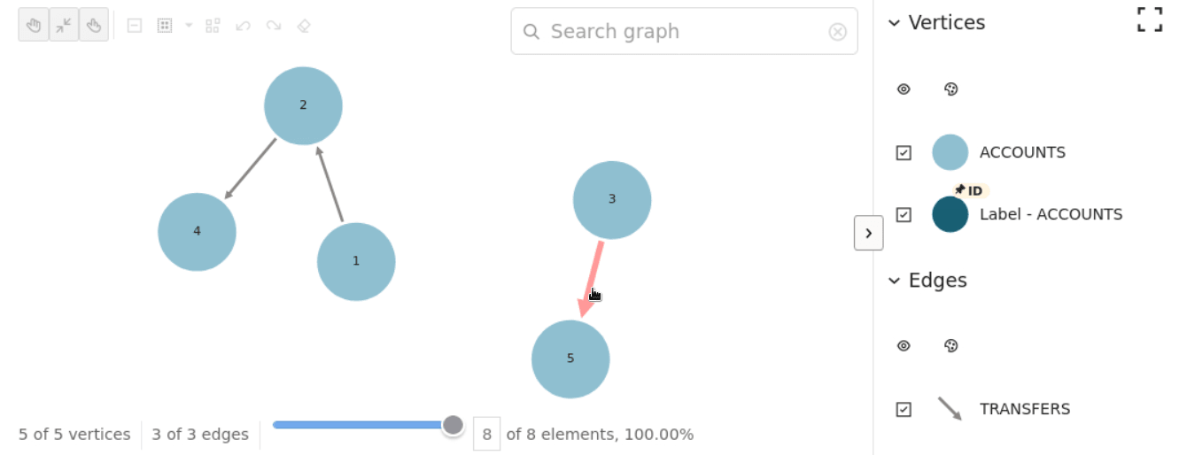
The preceding code produces the following graph visualization:

Figure 11-2 Graph Visualization with Custom Styling Options

Description of "Figure 11-2 Graph Visualization with Custom Styling Options"