Using the Jupyter Notebook Interface for PGQL Property Graphs

You can use the Jupyter notebook interface to create, load, and query PGQL property graphs through Python.

In addition, you can visualize PGQL property graphs using the graph visualization extension in both Jupyter Notebook and JupyterLab. See Getting Started with the Graph Visualization Extension in Jupyter Environments for more information.

The following steps show you how to create and visualize PGQL property graphs in a Jupyter environment (either Jupyter Notebook or JupyterLab).

1. Install the desired Jupyter Notebook interface (either Jupyter Notebook or JupyterLab).

2. Ensure that your Jupyter installation is added to the PATH environment variable.

3. Install the graph visualization extension in your Jupyter environment. See Installing the Graph Visualization Extension for Jupyter for more information.

4. Create and query a PGQL property graph using the OPG4Py Python API in a notebook cell using the following code.

   import opg4py;
   from pypgx import setloglevel
   from opg4py import graph_server
   setloglevel("ROOT", "WARN")
   
   pgql_conn = opg4py.pgql.get_connection("<username>","<password_for_user>","jdbc:oracle:thin:@<host_name>/<service>")
   pgql_statement = pgql_conn.create_statement()
   pgql = '''
       CREATE PROPERTY GRAPH bank_graph_pgql
         VERTEX TABLES (
           BANK_ACCOUNTS
             KEY ( ID )
             LABEL accounts PROPERTIES ( ID, name )
         )
         EDGE TABLES (
           BANK_TRANSFERS
             SOURCE KEY ( src_acct_id ) REFERENCES BANK_ACCOUNTS(ID)
             DESTINATION KEY ( dst_acct_id ) REFERENCES BANK_ACCOUNTS(ID)
             LABEL transfers PROPERTIES ( amount, description, src_acct_id, dst_acct_id, txn_id )
         ) OPTIONS(PG_VIEW)
   '''
   pgql_statement.execute(pgql

   Figure: Creating and Querying a PGQL property graph in Jupyter Notebook

   

   Description of the illustration jupyter_graph_on_db.png

5. Visualize the query results using PgqlGraphVisualization in oraclegraph Jupyter extension.

   1. Establish a connection to the database using the Python oracledb driver.

      import oracledb
      connection = connection=oracledb.connect(
      user=graphuser,
      password="<password_for_graph_user>",
      dsn="<hostname:port/dbservice>",
      print("Connection established successfully.")

   2. Run a PGQL query on your property graph and visualize the query results using the graph visualization extension.

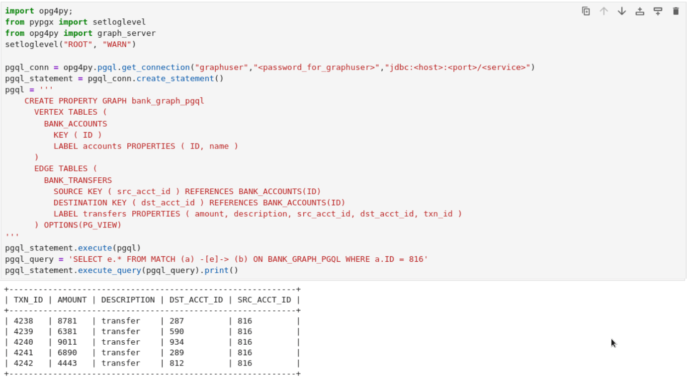
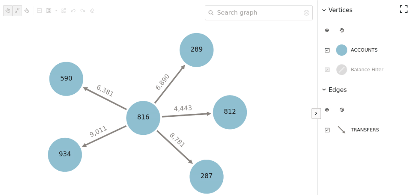
      For instance, the following example shows the graph visualization of a PGQL query on the property graph created at step-4 using PgqlGraphVisualization in the oraclegraph Jupyter extension.

      from pypgx import setloglevel
      from oraclegraph import GraphVisualization, PgqlGraphVisualization
      
      setloglevel('ROOT', 'WARN')
      
      vq = PgqlGraphVisualization("graphuser", "<password_for_graphuser>", "<host_name:port>/<service>")
      
      query='''
      SELECT * FROM GRAPH_TABLE (bank_graph_pgql
        MATCH (a) -[e]-> (b)
        WHERE a.ID=816
      COLUMNS (a.ID AS src_ac, e.AMOUNT AS amount, b.ID AS dest_ac)
      )
      '''
      graph_query = vq.visualize_query(query)
      
      defaults_feature = {
        "interactionActive": True,
        "1stickyActive": True
      }
      
      base_styles = {
        "vertex": {
          "label": "${properties.ID}",
          "size": 20
        },
        "edge": {
          "label": "${properties.AMOUNT}"
        }
      }
      
      rule_based_styles = [{
          "stylingEnabled": True,
          "component": "vertex",
          "target": "vertex",
          "conditions": {
            "conditions": [{
              "property": "BALANCE",
              "operator": "<=",
              "value": 5000
            }],
          },
          "style": {
            "color": "green"
          },
          "legendTitle": "Balance Filter",
          "legendDisplayed": True
        }
      
      ]
      
      settings = {
        "numberOfHops": 2,
        "showLegend": True,
        "defaults": defaults_feature,
        "baseStyles": base_styles,
        "ruleBasedStyles": rule_based_styles
      }
      bank_graph = GraphVisualization(data = graph_query, settings = settings)
      bank_graph.height = 600
      display(bank_graph)

      The preceding code produces the following visualization result:

      Figure: PGQl Property Graph Visualization

      

      Description of the illustration jupyter_pgql_viz.png

6. Load and analyze the property graph in the graph server (PGX).

   The following example shows loading the PGQL property graph into the graph server (PGX) and running graph algorithms for analysis:

   base_url = "https://localhost:7007"
   username = "graphuser"
   password = "<password_for_graphuser>"
   
   instance = graph_server.get_instance(base_url, username, password)
   session = instance.create_session('jupyter')
   graph = session.read_graph_by_name('BANK_GRAPH_PGQL', 'pg_pgql')
   analyst = session.create_analyst()
   analyst.pagerank(graph)
   rs = graph.query_pgql("SELECT id(x), x.pagerank FROM MATCH (x) LIMIT 5")
   rs.print()

   Figure: Running Graph Algorithms in Jupyter Notebook

   

   Description of the illustration jupyter_graph_analysis.png