3.2 The SQL Page
The SQL page enables you to enter and execute SQL and PL/SQL statements, and create database objects.
To navigate to the SQL page, do either of the following:
-
In the Lanuchpad page, click SQL.
-
Click Selector
 to display the navigation menu. Under Development, select
SQL.
You can use SQL and PL/SQL statements in the worksheet to create a table, insert data, create and edit a trigger, select data from a table, and save that data to a file. Some other features are syntax highlighting and error detection.
The SQL page consists of the left pane for navigating worksheets and objects, the editor for executing SQL statements, and the output pane for viewing the results. These panes are described in the following sections:
3.2.1 Navigating Objects and Worksheets
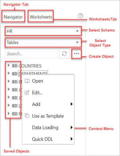
The Navigator tab in the left pane displays the saved objects for the selected schema.
The following figure shows the various elements in the left pane.
Figure 3-1 Left Pane in SQL
-
Schema and Object Type selector: Use the drop-down lists to select the schema and filter the results by the object type.
-
Worksheets tab: Displays the worksheets that are saved in the browser. You can open or delete an existing worksheet by using the context (right-click) menu.
Note:
The worksheets created are dependent on the browser used (Internet Explorer, Mozilla Firefox, or Google Chrome) for the session at the time of saving the worksheet, and they will not be accessible from any other browser. -
Search: Searches the contents of a saved worksheet or search for objects in the Navigator tab by name. The search functionality is not case-sensitive, retrieves all matching entries, and does not require the use of wild card characters.
-
Context menu: Options in the context menu are:
-
Open to browse properties and data relevant to the object type (tables and views).
The Data pane displays the data for a table, view, or materialized view.
To edit an entry, double-click a cell to make edits. You can also click
 and enter the value. When you make an edit, the border of the
gutter cell in that row changes to blue.
The icons available in the Data pane are:
- Create Row: Insert a new row into the database table. When you insert a row using the Create Row icon, the row is committed into the database.
-
Delete Selected: Mark the selected row for deletion. When you mark a row for deletion, the border of the row changes to red.
-
Commit: Commit all changes made to the database.
-
Undo All: Revert all changes that are marked for commit.
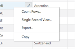
Use the Filter icon at the top right corner to filter the column data. You can also right-click a cell to access the context menu to count rows, view a single record, export or copy the cell text to clipboard.
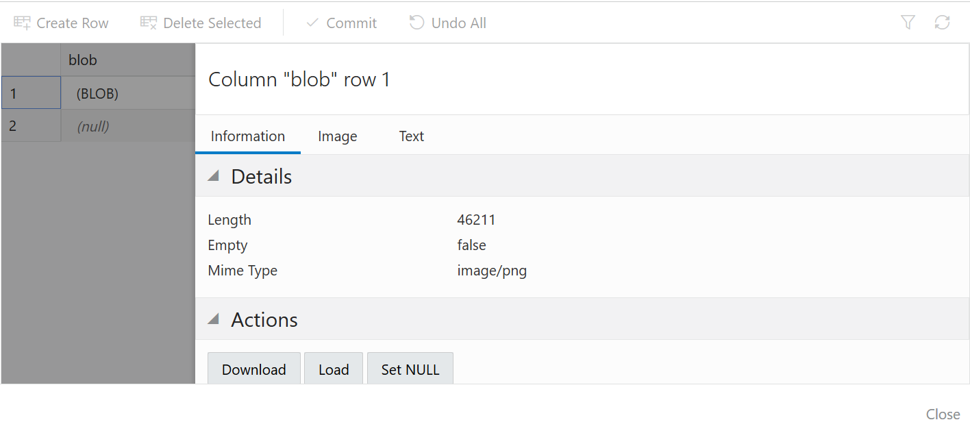
To view a Binary Large Object data type (BLOB), click the pencil icon for a BLOB data type. In the View Value dialog:- The Image tab displays the loaded image, if the loaded BLOB type is an image.
- The Text tab displays the text file, if the loaded BLOB type is text .
- The Information tab displays the details and allows you
to perform the following actions:
- Download: To download the image/text file of BLOB data type .
- Load: To insert an image/text of BLOB data type.
- Set NULL: To delete the object and set the value as NULL.
-
Edit edits the properties of an existing object.
-
Add creates an object based on the object type selected.
-
Use as Template creates an object by using the properties of an existing object as the template.
-
REST
-
Enable enables REST access for the database object. See Enabling REST Access for a Database Object
A REST enabled object is indicated by a REST Enabled icon
 in the Navigator tab.
-
Disable disables REST access for the database object after it is enabled. See Disabling REST Access for a Database Object
-
cURL Command generates a cURL call for a selected HTTP method for the database object. See Generating cURL Requests for a REST-Enabled Database Object
-
-
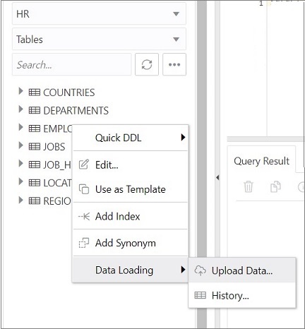
Data Loading loads data from local files into a table.
-
Quick DDL generates Data Definition Language statements for the object.
-
-
Refresh
 : Refreshes the objects or worksheets listed in the left pane.
-
Object Submenu
 : Opens the Create Object dialog to create a new object based on the
type selected in the drop-down list.
-
Help
 : Provides contextual help documentation.
You can drag objects from the left pane and drop them into the worksheet editor in the right pane.
-
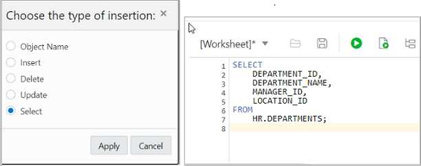
If you drag and drop a table or view, you are prompted to select one of the following SQL statements: Insert, Update, Select, or Delete. For example, if you choose Select, a Select statement is constructed with all columns in the table or view. You can then edit the statement, for example, modifying the column list or adding a WHERE clause.
If you choose Object Name, the name of the object prefixed by the schema name is added to the worksheet.
-
If you drag and drop a function or procedure, you can choose to insert the name or the PL/SQL code of the function or procedure in the worksheet. If you select the PL/SQL code, you can enter the parameters before inserting the code into the worksheet.
3.2.2 Executing SQL Statements in the Code Editor
The code editor in the SQL page enables you to run SQL and PL/SQL statements and scripts. The main features include in-context code completion, syntax highlighting, and error debugging.
You can enter SQL and PL/SQL statements to specify actions such as creating a table, inserting data, selecting data, or deleting data from a table. SQL keywords are automatically highlighted. For multiple statements, you must terminate:
- Each non-PL/SQL statement with either a semicolon (;) or a slash (/) on a new line
- Each PL/SQL statement with a slash (/) on a new line
For SQL*Plus and SQLcl statements supported in the worksheet, see Supported SQL*Plus and SQLcl Commands.
If you press Ctrl+Space, the editor provides you with a list of possible completions at the insertion point that you can use to autocomplete code that you are editing. This list is based on the code context at the insertion point.
The editor offers a comprehensive list of commands available through the Command Palette. To open the Command Palette, press Ctrl+Shift+P. For a list of keyboard shortcut keys, see Keyboard Shortcuts.
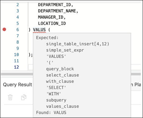
An error in the code is signified by a red dot in the left gutter and a squiggle line beneath the specific text. When you hover over it, you see a pop-up displaying possible fixes for resolving the error.
You can set code editor preferences using the Preferences option available in the top-right user drop-down list. Some of the code editor options that you can customize are Theme (Light, Dark and High contrast dark), Font size and family, Tab size, Word wrap, Ruler, Line numbers and so on.
The SQL toolbar contains icons for the following operations:
-
Worksheet enables you to create a worksheet, open or delete an existing worksheet, and save a worksheet.
Note:
The worksheets are saved in the browser. Therefore, if you do sensitive work on a computer in a public network, remember to clear the browser cache before you leave. Additionally, the saved worksheets will only be displayed in the browser that was used at the time of creating the worksheet. -
Run Statement executes the selected statements or the statement at the mouse pointer in the worksheet editor. The SQL statements can include bind variables and substitution variables of type VARCHAR2 (although in most cases, VARCHAR2 is automatically converted internally to NUMBER if necessary). A dialog box is displayed for entering variable values.
-
Run Script executes all statements in the worksheet editor using the Script Runner. The SQL statements can include bind variables (but not substitution variables) of type VARCHAR2 (although in most cases, VARCHAR2 is automatically converted internally to NUMBER if necessary). A dialog box is displayed for entering bind variable values.
- Create Chart creates a chart for the
corresponding SQL statement entered in the editor. In contrast, you
can partially highlight a subquery and create a chart. A slider
window is displayed for entering the chart parameters. For a
description of the fields, see Creating a Chart.
If the SQL statement is syntactically incorrect or incomplete, an error/warning notification is displayed.
-
Explain Plan generates the execution plan for the statement (internally executing the EXPLAIN PLAN statement). The execution plan is automatically displayed in the Explain Plan tab in the worksheet output pane.
-
Autotrace runs the statement and collects run time statistics and the actual execution plan. The Autotrace output is displayed in the Autotrace tab in the worksheet output pane. Currently, there are no preferences available.
-
Download Editor Content downloads the content of the worksheet as a SQL file to the local system.
-
Format formats the SQL statement in the editor, such as capitalizing the names of statements, clauses, keywords, and adding line breaks and indentation.
-
Clear removes the statements from the editor.
-
Tour provides a guided tour of the worksheet highlighting salient features and providing information that is useful if you are new to the interface.
-
Help provides context-related help and provides a link to the help documentation.
3.2.2.1 Keyboard Shortcuts
This section lists the keyboard shortcuts for various commands in the SQL page.
Table 3-1 Keyboard Shortcuts
| Windows | MacOS | Description |
|---|---|---|
|
Ctrl + Enter |
Cmd + Enter |
Runs the code as query. |
|
Ctrl + Down Arrow |
Cmd + Down Arrow |
Moves to the next SQL code from history. |
|
Ctrl + Up Arrow |
Cmd + Up Arrow |
Moves to the previous SQL code from history. |
|
Ctrl + S |
Cmd + S |
Saves the current worksheet. |
|
Ctrl + O |
Cmd + O |
Opens the worksheet browser dialog. |
|
Ctrl + I |
Cmd + I |
Downloads the content of the editor. |
| F1 | Fn + F1 | Opens the help topic. |
|
F5 |
Fn + F5 |
Runs code as script. |
|
F6 |
Fn + F6 |
Shows Autotrace. |
|
F10 |
Fn + F10 |
Shows Explain Plan. |
|
F11 |
Fn + F11 |
Creates a chart. |
|
Ctrl + B |
Cmd + B |
Opens the "Convert Case" drop-down list. |
|
Ctrl + F7 |
Cmd + Fn + F7 |
Formats code in the editor. |
|
Ctrl + Space |
Ctrl + Space |
Autocompletes code (shows hints). |
The following table lists the keyboard shortcuts for commands in the Command Palette.
Table 3-2 Command Palette Keyboard Shortcuts
| Windows | MacOS | Description |
|---|---|---|
| Ctrl + Alt + Up | Cmd + Option + Up | Add Cursor Above |
| Ctrl + Alt + Down | Cmd + Option + Down | Add Cursor Below |
| Shift + Alt + I | Shift + Option + I | Add Cursors to Line Ends |
| Ctrl + K Ctrl + C | Cmd + K Cmd + C | Add Line Comment |
| Ctrl + D | Cmd + D | Add Selection To Next Find Match |
| Shift + Alt + Down | Shift + Option + Down | Copy Line Down |
| Shift + Alt + Up | Shift + Option + Up | Copy Line Up |
| Ctrl + U | Cmd + U | Cursor Undo |
| Cmd + Backspace | Delete All Left | |
| Ctrl + K | Delete All Right | |
| Ctrl + Shift + K | Shift + Cmd + K | Delete Line |
| Shift + Alt + Right | Shift + Ctrl + Cmd + Right | Expand Selection |
| Ctrl + F | Cmd + F | Find |
| Enter | Enter | Find Next |
| Ctrl + F3 | Cmd + Fn + F3 | Find Next Selection |
| Shift + Enter | Shift + Enter | Find Previous |
| Ctrl + Shift + F3 | Shift + Cmd + Fn + F3 | Find Previous Selection |
| Cmd + E | Find With Selection | |
| Ctrl + Shift + [ | Option + Cmd + [ | Fold |
| Ctrl + K Ctrl + 0 | Cmd + K Cmd + 0 | Fold All |
| Ctrl + K Ctrl + / | Cmd + K Cmd + / | Fold All Block Comments |
| Ctrl + K Ctrl + 8 | Cmd + K Cmd + 8 | Fold All Regions |
| Ctrl + K Ctrl + 1 | Cmd + K Cmd + 1 | Fold Level 1 |
| Ctrl + K Ctrl + 2 | Cmd + K Cmd + 2 | Fold Level 2 |
| Ctrl + K Ctrl + 3 | Cmd + K Cmd + 3 | Fold Level 3 |
| Ctrl + K Ctrl + 4 | Cmd + K Cmd + 4 | Fold Level 4 |
| Ctrl + K Ctrl + 5 | Cmd + K Cmd + 5 | Fold Level 5 |
| Ctrl + K Ctrl + 6 | Cmd + K Cmd + 6 | Fold Level 6 |
| Ctrl + K Ctrl + 7 | Cmd + K Cmd + 7 | Fold Level 7 |
| Ctrl + K Ctrl + [ | Cmd + K Cmd + [ | Fold Recursively |
| Ctrl + Shift + \ | Shift + Cmd + \ | Go to Bracket |
| Ctrl + G | Ctrl + G | Go to Line... |
| Alt + F8 | Option + Fn + F8 | Go to Next Problem(Error, Warning, Info) |
| F8 | Fn + F8 | Go to Next Problem in Files (Error, Warning, Info) |
| F7 | Fn + F7 | Go to Next Symbol Highlight |
| Shift + Alt + F8 | Shift + Option + Fn + F8 | Go to Previous Problem (Error, Warning, Info) |
| Shift + F8 | Shift + Fn + F8 | Go to Previous Problem in Files (Error, Warning, Info) |
| Shift + F7 | Shift + Fn + F7 | Go to Previous Symbol Highlight |
| Ctrl + ] | Cmd + ] | Indent Line |
| Ctrl + Shift + Enter | Shift + Cmd + Enter | Insert Line Above |
| Ctrl + J | Join Lines | |
| Ctrl + K Ctrl + D | Cmd + K Cmd + D | Move Last Selection To Next Find Match |
| Alt + Down | Option + Down | Move Line Down |
| Alt + Up | Option + Up | Move Line up |
|
F1 (All browsers) Ctrl + Shift + P (Google Chrome only) |
Fn + F1 | Open Command palette |
| Ctrl + [ | Cmd + [ | Outdent Line |
| Ctrl + K Ctrl + U | Cmd + K Cmd + U | Remove Line Comment |
| Ctrl + H | Option + Cmd + F | Replace |
| Ctrl + Shift + . | Shift + Cmd + . | Replace with Next Value |
| Ctrl + Shift + , | Shift + Cmd + , | Replace with Previous Value |
| Ctrl + Shift + L | Shift + Cmd + L | Select All Occurrences of Find Match |
| Alt + F1 | Option + Fn + F1 | Show Accessibility Help |
| Shift + F10 | Shift + Fn + F10 | Show Editor Context Menu |
| Ctrl + K Ctrl + I | Cmd + K Cmd + I | Show Hover |
| Shift + Alt + Left | Shift + Ctrl + Cmd + Left | Shrink Selection |
| Shift + Alt + A | Shift + Option + A | Toggle Block Comment |
| Ctrl + K Ctrl + L | Cmd + K Cmd + L | Toggle Fold |
| Ctrl + / | Cmd + / | Toggle Line Comment |
| Ctrl + M | Shift + Ctrl + M | Toggle Tab Key Moves Focus |
| Shift + Ctrl + T | Transpose Letters | |
| Ctrl + Space | Ctrl + Space | Trigger Suggest |
| Ctrl + K Ctrl + X | Cmd + K Cmd + X | Trim Trailing Whitespace |
| Ctrl + Shift + ] | Option + Cmd + ] | Unfold |
| Ctrl + K Ctrl + J | Cmd + K Cmd + J | Unfold All |
| Ctrl + K Ctrl + 9 | Cmd + K Cmd + 9 | Unfold All regions |
| Ctrl + K Ctrl + ] | Cmd + K Cmd + ] | Unfold Recursively |
3.2.3 Viewing the SQL Output
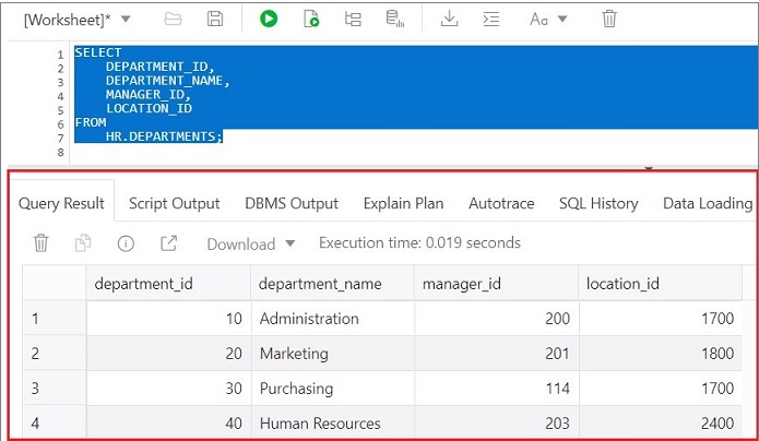
The lower right pane in SQL displays the output of the operation executed in the SQL editor.
The following figure shows the output pane in the SQL page.
The output pane has the following tabs:
-
Query Result: Displays the results of the most recent Run Statement operation in a display table.
-
Script Output: Displays the text output from your statements executed as a script using the script engine.
-
DBMS Output: Displays the output of DBMS_OUTPUT package statements.
-
Explain Plan: Displays the plan for your query using the Explain Plan command.
-
Autotrace: Displays the session statistics and execution plan from
v$sql_planwhen executing a SQL statement using the Autotrace feature. Displays the output if you clicked the Autotrace icon. -
SQL History: Displays the SQL statements and scripts that you have executed. To re-enter a previously executed query in the worksheet, double-click the query in the history list. You can search for specific statements by clicking the Search icon. The Search functionality is case-sensitive, retrieves all entries that contain the search text, and does not require wildcard characters.
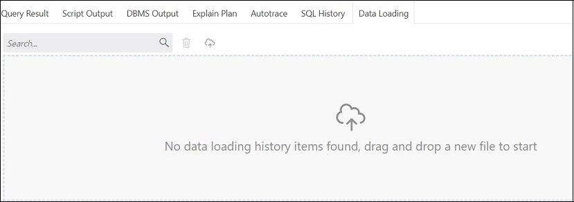
- Data Loading: Displays a report of the total rows loaded and failed for all visible tables (including tables from other schemas).
The icons in this pane are:
-
Clear output: Clears the output.
-
Show info: Displays the SQL statement for which the output is displayed.
-
Open in new tab: Opens the query result or explain plan in a new window.
-
Download: This is applicable only for Query Result. Enables you to download the query result to your local computer in CSV, JSON, XML, or TEXT (.tsv) format.
In the Query Result tab, in the display table, the context menu (right-click) for the row header consists of the following:
-
Columns enables you to select columns to hide.
-
Sort displays a dialog box for selecting columns to sort by. For each column, you can specify ascending or descending order, and you can specify that null values be displayed first.
The context menu for the rest of the display table consists of the following commands:
-
Count Rows displays the number of rows in the result set for your query.
-
Single Record View enables you to view data for a table or view, one record at a time.
-
Export generates the file for download based on the format selected, which can be XML, CSV (comma-separated values including a header row for column identifiers), Insert , Delimited, Fixed, HTML, JSON, or TEXT.
-
Format: Select the format to export from the drop-down list.
-
Line Terminator: Identifies the terminator for each line. The line terminator is not included in the data exported. If the preview page shows the data in one single row, the correct terminator is not specified.
-
Header: Controls whether the first row is a header row or the first row of data.
-
Left and Right Enclosure: Enclosures are used for character data and are optional. Enclosures are not included in the data exported.
Note:
If a popup blocker is enabled, it will prevent the file from downloading. -
-
Copy copies data from a cell or a row or a range of rows.
3.2.4 Loading Data
In the SQL page, you can load data from a local file into an existing table or into a new table.
The file formats that you can load are CSV, XLS, XLSX, TSV, TXT, XML, JSON, and AVRO. For XML, JSON, and AVRO files, see Format Specifications for JSON, AVRO, and XML Files.
3.2.4.1 Loading Data from a Local File to a New Table
To load data from a local file to a new table:
-
You can start in one of the following ways:
-
In the Navigator tab, in the left pane, click Object submenu
 , select Data Loading, and then select Upload Data into New
Table.
Figure 3-6 Upload Data to New Table Option

Description of "Figure 3-6 Upload Data to New Table Option" -
In the Navigator tab, drag and drop the local file into the left pane. When you drag a file into the pane, the following message is displayed Drop the file here to start.
-
In the worksheet output pane, select the Data Loading tab and drag and drop the local file into the output pane.
The Upload Data into New Table is displayed. A preview of the data is displayed in a grid format.
-
-
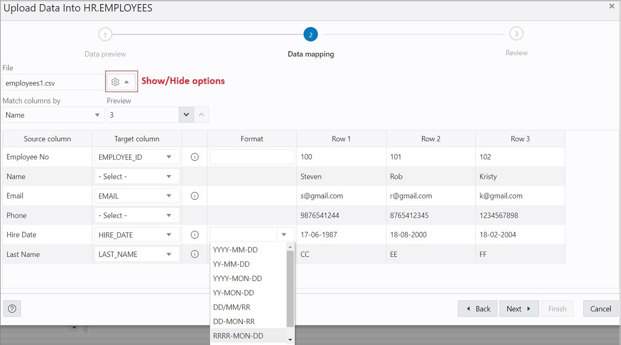
Click Show/Hide options
 to display options that you can modify for data preview:
-
Column names: Select Get from file to display column headers in the first row.
- Encoding: An option to select the encoding type is visible when the loaded file is in plain text format (CSV, TSV, or TXT). The default encoding type is UTF-8.
-
Text enclosure and Field delimiter: These options are visible only when the selected file is in plain text format (CSV, TSV, or TXT). Select or enter the character used in the source file for text enclosure and field delimiter.
-
Rows to skip: Enter or use the up and down arrows to select the number of rows to skip.
-
Preview size: Enter or use the up and down arrows to select the number of rows to preview.
-
Limit rows to upload: If you select this option, you need to specify the rows to load. Use the up and down arrows to select the number of rows to load.
To remove the options selected and the data preview, click Clear.
After selecting the required options, click Apply, and then click Next.
-
-
In Table Definition, do the following:
-
In the Table Name field, enter a name for the target table.
-
Select the check box at the beginning of a row to add the column to the target table.
-
Select or enter values for column attributes such as Column Name, Column Type, Precision, Scale, Default, Primary Key and Nullable.
-
The Format Mask column appears for date, timestamp and numeric types of data. For date and timestamp types, you must select a value from the drop-down list or type the value in the Format Mask field. For numeric types, the format mask is optional.
For a date and timestamp column, you need to supply a compatible format mask that describes the data being uploaded. For example, if the date data looks like
12-FEB-2021 12.21.30, you need to supply a date mask ofDD-MON-YYYY HH.MI.SS. The format mask is automatically determined based on the data in the file. You need to review the suggested format mask and if needed, modify it by entering the format directly into the target cell.
Figure 3-8 Table Definition Step in Upload Data into New Table
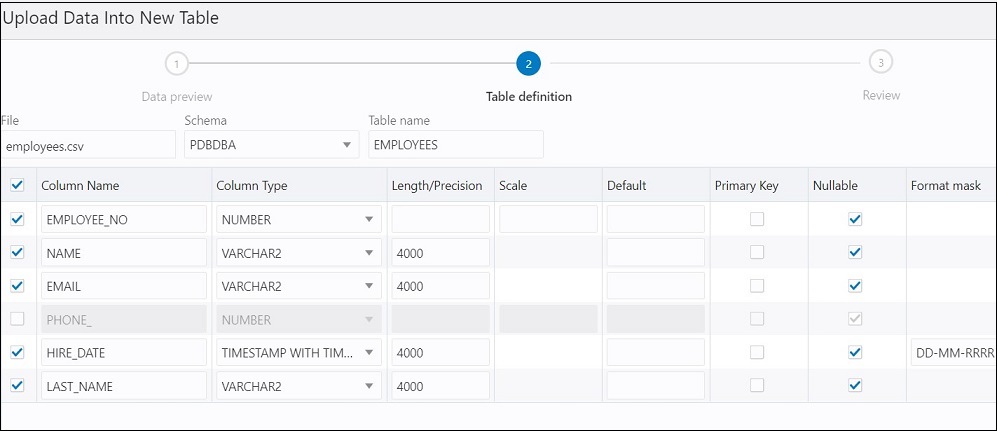
Description of "Figure 3-8 Table Definition Step in Upload Data into New Table"Click Next.
-
-
Review the generated DDL code based on the selections made in the previous screens. The mapping of the source to target columns are also displayed.
Click Finish. After the data is successfully loaded, the new table is displayed in the Navigator tab.
- For a detailed report of the total rows loaded and failed,
do one of the following:
-
Right-click the table in the Navigator tab, select Data Loading, and then select History. This displays the report for a specific table.
-
In the Navigator tab, select Object submenu
 , select Data Loading, and then select History. This displays
the report for all tables in the schema that is selected in the Navigator tab.
-
In the worksheet output pane, select the Data Loading tab. This displays the report for all visible tables (including tables from other schemas).
A summary of the data loaded is displayed in the History dialog. If any data failed to load, you can view the number of failed rows in the Failed Rows column. Click the failed rows column to open a dialog showing the failed rows.
In the History dialog, you can also search for files loaded by schema name, table name, or file name. To remove the loaded files, click Remove all history
 .
.
-
3.2.4.2 Loading Data from a Local File to an Existing Table
To load data from a local file to an existing table:
3.2.4.3 Format Specifications for JSON, AVRO, and XML Files
Data has to be stored in a particular format for JSON, AVRO, and XML files to load them successfully into a table.
The format specifications are described in the following sections.
3.2.4.3.1 JSON and AVRO Files
For JSON and AVRO files, the conversion for primitive types to table columns is supported only for top-level data. Nested objects are saved as JSON strings such as VARCHAR2 (JSON) or CLOB (JSON).
Note:
JSON check constraints are available only for Oracle Database 12c and later releases.
Consider the following JSON file as an example:
[
  {
    "ItemNumber": 1,
    "Description": "One Magic Christmas",
    "Part": {
      "UnitPrice": 19.95,
      "UPCCode": 13131092899
    },
    "Quantity": 9,
    "Total": 179.55
  },
  {
    "ItemNumber": 2,
    "Description": "Lethal Weapon",
    "Part": {
      "UnitPrice": 17.95,
      "UPCCode": 85391628927
    },
    "Quantity": 5,
    "Total": 89.75
  }
]
The AVRO schema for this file:
{
     "type": "array",
     "items": {
          "type": "record",
          "fields": [
               {
                    "name": "ItemNumber",
                    "type": "int"
               },
               {
                    "name": "Description",
                    "type": "string"
               },
               {
                    "name": "Part",
                    "type": {
                         "type": "record",
                         "fields": [
                              {
                                   "name": "UnitPrice",
                                   "type": "float"
                              },
                              {
                                   "name": "UPCCode",
                                   "type": "float"
                              }
                         ]
                    }
               },
               {
                    "name": "Quantity",
                    "type": "int"
               },
               {
                    "name": "Total",
                    "type": "float"
               }
          ]
     }
}
Load the JSON file using "Upload Data" in the SQL page, and it is converted
to the following table with two rows. part is a nested object that is
assigned the column type CLOB (JSON) during data mapping.
3.2.4.3.2 XML Files
This section lists the specifications for loading XML files.
-
Attributes will have their own columns
If the XML data is structured as:
<?xml version="1.0"?>
<catalog>
  <book id="bk102">
    <author>Ralls, Kim</author>
    <title>Midnight Rain</title>
    <genre>Fantasy</genre>
    <publisher>John Doe</publisher>
   </book>
</catalog>
The generated columns in the table are
id,author,title,genre, andpublisher. -
Two or more levels of nesting are needed to parse the data
In the following example, the data that needs to be parsed will not be located because it has only one level of nesting (catalog).
<?xml version="1.0"?>
<catalog>
  <author>Ralls, Kim</author>
  <title>Midnight Rain</title>
  <genre>Fantasy</genre>
  <publisher>John Doe</publisher>
</catalog>
However, the following examples will work:
<?xml version="1.0"?>
<catalog>
  <book id="bk102">
    <author>Ralls, Kim</author>
    <title>Midnight Rain</title>
    <genre>Fantasy</genre>
    <publisher>John Doe</publisher>
  </book>
</catalog>
or
<?xml version="1.0"?>
<catalog>
  <bookstore>
    <book id="bk102">
      <author>Ralls, Kim</author>
      <title>Midnight Rain</title>
      <genre>Fantasy</genre>
      <publisher>John Doe</publisher>
    </book>
  </bookstore>
</catalog>
or
<?xml version="1.0"?> <catalog> <bookstore> <shelf> <book id="bk102"> <author>Ralls, Kim</author> <title>Midnight Rain</title> <genre>Fantasy</genre> <publisher>John Doe</publisher> </book> </shelf> </bookstore> </catalog> -
Special characters such as hyphen (-) and period (.) in tag names are replaced by underscore (_) in the column name
XML tag names can contain hyphens and periods. Since the parser is converting XML to JSON, these characters become invalid object keys.
<?xml version="1.0"?>
<catalog>
  <book id="bk102">
    <author-name>Ralls, Kim</author-name>
    <title.1>Midnight Rain</title.1>
    <genre>Fantasy</genre>
    <publisher>John Doe</publisher>
   </book>
</catalog>
The generated columns are
id,author_name,title_1,genre, andpublisher. -
First-level only-text tags are ignored
<?xml version="1.0"?>
<catalog>
  <library> New Age Library </library>
  <book id="bk102">
    <author>Ralls, Kim</author>
    <title>Midnight Rain</title>
    <genre>Fantasy</genre>
    <publisher>John Doe</publisher>
  </book>
</catalog>
The
<library>tag is ignored and only the content of the<book>tag is taken into account. The generated columns areid,author,title,genre, andpublisher. -
First-level repetitive data is interpreted as an array of values
<?xml version="1.0" encoding="UTF-8"?>
<items id="orders">
    <item_number>1</item_number>
    <description>One Magic Christmas</description>
    <part>
      <unit_price>19.95</unit_price>
      <upccode>13131092899</upccode>
    </part>
    <quantity>9</quantity>
    <total>179.55</total>
    <item_number>2</item_number>
    <description>Lethal Weapon</description>
    <part>
      <unit_price>17.95</unit_price>
      <upccode>85391628927</upccode>
    </part>
    <quantity>5</quantity>
    <total>89.75</total>
</items>
The generated columns include
item_number,description,part, and each column will have only one row with the following values respectively ([1,2], ["One Magic Christmas","Lethal Weapon"], [{" unit_price":19.95,"upccode":13131092899},{"unit_price":17.95,"upccode":85391628927}] and so on for the remaining columns. -
Tags containing values and attributes are converted to object
<?xml version="1.0"?>
<catalog>
  <book id="bk102">
    <author country="ca">Ralls, Kim</author>
    <title>Midnight Rain</title>
    <genre>Fantasy</genre>
    <publisher>John Doe</publisher>
  </book>
</catalog>
The
<author>tag is converted to a column and will have an object as value that is structured as:{ "_":"Ralls, Kim", "country":"ca" }Note that the value of the tag has underscore ("_") as key and the attributes as "attribute_name": "attribute_value".
