22.2 Defining a Model
To define a model, follow these steps:
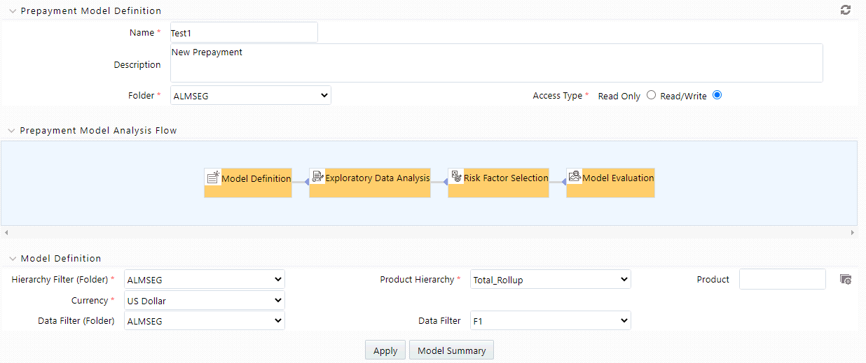
- Navigate to Prepayment Model Analysis window. Click Add .
The Definition window is displayed.
Figure 22-1 Prepayment Model Analysis
- Enter the following details.
Table 22-4 Form Fields to define a Model
Fields Description Name Enter the name of Prepayment Model Analysis rule Description Enter the description of Prepayment Model Analysis rule Folder Select the folder where you want to save Prepayment Model Analysis rule Access Type Select Access Type as Read-only or Read/Write. Hierarchy Filter (Folder) Select the folder of Hierarchy Filter. Product Hierarchy Select the Product Hierarchy. Product Based on the selected product hierarchy in model definition UI, Hierarchy Browser will expand the product hierarchy and you can select any parent/leaf node by clicking on the view button next to the product in the model definition screen. Currency Select the currency for the Prepayment Model Analysis rule. Default Currency option is also given, if you want to select the product irrespective of currency in which deal is booked. Data Filter (Folder) Select the folder name of data filter for Prepayment Model Analysis rule Data Filter Select the data filter to define the portfolio at more granular level than just, product and currency combination. - Click Apply to navigate to Exploratory Data Analysis window.
- Exploratory Data Analysis window is used to perform EDA
calculations.
Figure 22-2 Exploratory Data Analysis

Enter the following details in Exploratory Data Analysis window.
Table 22-5 Form Fields of Exploratory Data Analysis window
Fields Description Sample Size Sample size of dataset for EDA Model Population (As of Date Range) You can define a date range within which one wants to use data for model creation as model population.
By Default, Date range would be populated as below:
End Date: Max (As of Date) available in Model input Table
Start Date: Max [min (As of Date), End Date – 10 Years]
Do Sampling Select this option to create model based on a data Sample rather than the whole population. By default, Do Sampling is enabled. This would enhance performance due to lesser number of records considered for modelling, without degrading model quality. Sample Size (Multiplier) After selecting sample size for EDA, you can select multiplier value. This indicates sample size required for model creation. For example, if 1000, records are selected as sample size for EDA, and multiplier is 6, then a minimum of 1000*6 = 6000 records would be required for model creation.
Note: This checkbox is enabled only if Do Sampling checkbox is selected.
- This window gives complete information about all the risk factors along with
prepayment rates. It helps you do decide what all factors could influence the
customer’s prepayment behavior and would be best for model building.
You can hover over any graph and zoom in to enhance the visibility of the graph.
Click Model Summary to navigate back to the Model Summary window after saving all inputs/EDA graphs defined/generated till this point.
Click Re-Calculate if you want to change the sample size and redo the EDA again. change the sample size and click Re-Calculate.
If you have performed EDA multiple times (for example, three versions V1, V2, V3.), then use Versions (EDA) to view them. For example, when you are on the EDA screen and performing the EDA 3rd time, but still want to go with the 2nd EDA version, then select that version and subsequent processing would be based on V2. If you have run the EDA only once, then this drop-down will not be available.
When you hover over Sample size for EDA, it displays Default value (callout) as Default Value is 5000.
- Click Pair Plot to generate Pair Plot/Grid along with other EDA graphs. Pair Plot/Grid is a detailed graph, that can further slow down the processing. So you can explicitly select the pair plot checkbox and click on calculate to perform the EDA.
- Click Next. The Risk Factor Selection window is displayed. By
default, all the risk factors will be disabled.
Figure 22-3 Risk Factor Selection window
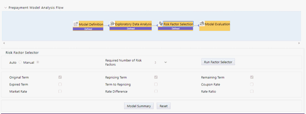
- You can change the risk factor selection mode to ‘Manual’ and all the risk factors
would be available for selection; maximum 3 factors can be selected after that all
the risk factors would be disabled again.
When you are in Auto Select Mode, System would perform required calculations, co-relation/collinearity analysis in the backend based on the required number of risk factors (Maximum 3), System would auto-select the best representative set of risk factors as per the input data.
If you want to change sample size and re-calculate EDA again, click Exploratory Data Analysis block and perform EDA with updated sample size. Again, the process starts from that step onwards, and updated EDA plots/graphs would be saved for the model.
- Click Next to navigate to Model Evaluation window. A confirmation
message is displayed. Click OK.
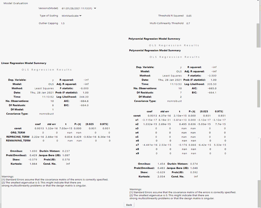
Figure 22-4 Model Evaluation
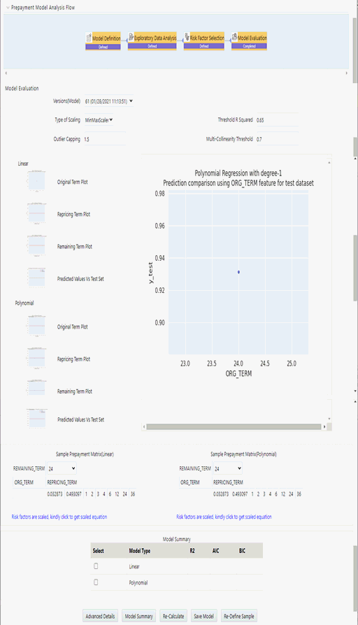
- Click Calculate to view all the evaluation parameters and quality plots.
- Click Re-Calculate if you are not satisfied with the model quality to
change the model parameters and revise the model definition. You can zoom the graph
to enhance visibility.
If you are changing parameters and generating different versions of the model, then you can see all the versions, generated with different set of model parameters in the Versions (Model) drop-down. If you have run “model evaluation’ only once, then this drop-down would not be available. As per the selected version, the Advanced model details window is also updated. The Model Details window helps you to evaluate the model fit. It has the following comparisons:
Predicted Values Vs Risk Factor 1,2,3, as per the number of risk factors considered for model building. This will dynamically adjust as per the number of risk factors selected.
Predicted Values Vs Test Sample.
Sample prepayment matrix as per both the models (Linear and Polynomial).Figure 22-5 Sample prepayment matrix

User would have option to redefine, values for sample matrix by clicking on “Re-define Sample” button. Below pop up would open up if user would like to re-define sample buckets. Again this pop up would dynamically adjust based on number of risk factors selected in the model.
- Click Model Summary to view Model Summary window, after saving all details.
- Click Re-Define Sample if you want to modify risk factor values
for sample matrix. This pop up would dynamically adjust to display 1,2 or 3
dimensions as per the chosen model.
Figure 22-6 Risk factor values
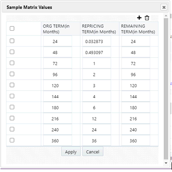
In case you want to update values on which sample matrix is generated, you can click on ‘Re-define Sample’. Below window would open up where you can update the risk factor values:
Add row using Add +. You can add multiple rows or delete multiple rows using buttons in panel 1. Default sample matrix is10*10, but once you re-define sample, matrix can be truncated to any dimensions.
The redefined matrix will be saved along with model.
Model summary parameters like R2, AIC and BIC.
Both (Linear/Polynomial) models are produced when the system compares model generated R2 against the R2 threshold defined by the user. The final option is given to you to choose any one of these models. Based on infrastructure availability and model complexity, user can choose any one of linear/polynomial model.
Click Save Model to save the model. Same model could be referred to populate prepayment rate matrix.
Click Re-Calculate to re-evaluate model based on changed model parameters.
If you want to change sample size and re-calculate EDA again, click Exploratory Data Analysis block and perform EDA with updated sample size. Again, process would start from that step onwards and updated EDA plots/graphs would be saved for the model.
If you want to update selected risk factors, click Risk Factor Selection block and change risk factors. Again, process would start from that step onwards and updated risk factors would be saved for the model.
Figure 22-7 Advance Details
Reset button on each screen would help to delete all the calculations done in subsequent steps. That is, if you have done EDA and selected particular EDA version to do further calculations like ‘Risk factor Selection’ or ‘Model Evaluation’. In case you are not satisfied with model, you can go back to EDA, click ‘Reset’ to clear out the details/calculations performed in subsequent stages and do recalculate with a different set of parameters.
Following are the default values/usage of Parameters:
Default values/usage of Parameters
| Parameters | Default Values |
|---|---|
| EDA Sample Size | This would allow you to define a sample size for exploratory data analysis. A bigger sample would increase CPU and memory usage, but it would better represent the model population. You have the option not to use sampling by setting Do_Sampling parameter to false. Procedure for the same is given in next section. |
| Type of scaling |
Many a times, risk factors are not in consistent range, e.g. one of the risk factor’s values could be in 1-500 range but another risk factor could be just in 2-3 range. So, risk factor 1 would influence the model more and you would get a biased model. So, to make all the risk factors consistent, scaling is used. There are two types of scaling: Min-Max Scaling = (X – min)/(max – min) Standard = (X – Mean)/Std. Deviation |
| Threshold R2 | R-squared values range from 0 to 1 and are commonly stated as percentages from 0% to 100%. An R-squared of 100% means that all movements of prepayment rate (dependent variable) are completely explained by movements in the chosen risk factors (independent variable(s). |
| Multi-collinearity Threshold | For model creation if two risk factors/variables are highly correlated or correlation > 0.7, they would make model unstable. So based on this value, if variables are highly correlated or above defined threshold, one of them would be dropped while model creation. |
| Outlier Capping | This would allow user to reject values beyond certain percentile. Sometimes, input data has few extreme values which could distort the model. So you could reject those values and get a stable model. |
Exploratory Data Analysis:
Sample Size (EDA) - 5000
Model Population Range - It would be auto-populated based on the data in risk factor table. Maximum would be 10 years older from latest available date. In case you think, older data is not relevant, as of date range can be updated.
Model Evaluation:
Type of scaling – min Max Scaler
Threshold R2 – 0.65
Outlier capping – 1.5 Percentile
Multi-collinearity Threshold – 0.7