13.9.1.1 An Example: Product Versus Balance Sheet Level Results

Let us assume that for the 1 Liability Instrument, Oracle ALM calculates a Market Value of $100,000 and the following accrued Dynamic Present Values for each scenario:

Table 13-5 Dynamic Present Values for each Scenario

Scenario	Accrued Dynamic Present Value
1	126,408
2	124,773
3	91,192
4	82,043
5	76,851

Though the actual value to the bank is -$100,000, Oracle ALM by convention reports a positive market value for all instruments. Therefore, it is important to remember that positive market value for liability is in effect a loss. The same convention applies to VaR. Though VaR is defined as the "maximum loss (to the bank)", it must be substituted with “maximum gain (to the bank)” when interpreting the VaR output for an instrument that is a liability.

Assume Oracle ALM outputs the first three columns of the following table to the FSI_O_STOCH_VAR table for the 1 liability product. Recall that FSI_O_STOCH_VAR contains product level output. When interpreting the VaR output for liability on a product output level, you must remember that VaR is the "maximum gain (to the bank)".

Table 13-6 List of VaR output for Liability

Scenario	Probability	VaR	Interpretation
1	0.2	100,000 -126,408 = -26,408	With a prob. of 20%, gain ≤ -26,408
2	0.4	100,000 -124,773 = -24,773	With a prob. of 40%, gain ≤ -24,773
3	0.6	100,000 -91,192 = 8,808	With a prob. of 60%, gain ≤ 8,808
4	0.8	100,000 -82,043 = 17,957	With a prob. of 80%, gain ≤ 17,957
5	1.0	100,000 -76,851 = 23,149	With a prob. of 100%, gain ≤ 23,149

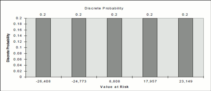
The discrete probability of a gain of exactly -$26,408, -$24,733, $8,808, $17,957, $23,149 is 20% for a 5 scenarios simulation.

Note:

The sum of all probabilities adds up to a total of 100% probability.

Figure 13-3 Graph of Discrete Probability

Description of graph of Discrete Probability follows:

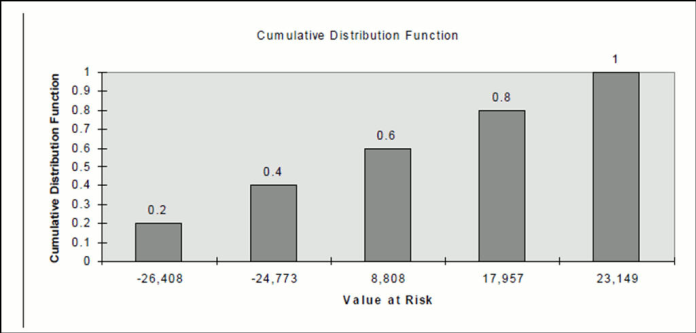
In Value at Risk interpretation, we need to convert the discrete probability to a cumulative distribution function. For example, we know that there is a chance of a gain of -$26,408 with a probability of 20% and a gain of -$24,773 with a probability of 20%. This means that there is a 40% probability of gain less than or equal to -$24,773. This comes from adding a 20% discrete probability from the gain of $-26,408 and a 20% discrete probability from a gain of -$24,773.

Figure 13-4 Graph of Cumulative Distribution Program

Description of graph of Cumulative Distribution function follows:

Now let us assume Oracle ALM outputs the first three columns of the following table to FSI_O_STOCH_TOT_VAR table for the 1 liability product. Recall that FSI_O_STOCH_TOT_VAR contains a balance sheet level output. At the balance sheet level, we aggregate gain/loss information for different products that can be either assets or liabilities. Oracle ALM by convention reports the aggregated VaR number as a “maximum loss”; therefore, the sign of VaR for all liabilities must be reversed.

Table 13-7 List of VaR Liabilities

Scenario	Probability	VaR	Interpretation
5	0.2	-23,149	With a prob. of 20%, loss ≤ -23,149
4	0.4	-17,957	With a prob. of 40%, loss ≤ -17,957
3	0.6	-8,808	With a prob. of 60%, loss ≤ -8,808
2	0.8	24,773	With a prob. of 80%, loss ≤ 24,773
1	1.0	26,408	With a prob. of 100%, loss ≤ 26,408