13.9.2 Validating Interpretation

Let us analyze the most beneficial scenario (to the bank) to prove that our interpretation is correct. In scenario 5, the “gain = 23,149” has a probability of 20% because it is a discrete event. We also have the following events and probabilities:

Table 13-8 Events and Probabilities

Event	Probability
gain < 23,149	80%
gain = 23,149	20%
gain > 23,149	0

Note:

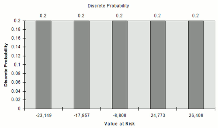
When we apply the signage to liability, the discrete probability is undisturbed for each event.

Figure 13-5 Discrete Probability

Description of graph of Discrete Probability follows:

We see here that there is a 20% probability of a maximum loss of -$23,149. There is a 40% probability of a maximum loss of -$23,149 (20% discrete probability from -$23,149 plus 20% discrete probability from -$17,957).

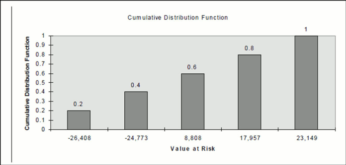
Figure 13-6 Cumulative Distribution Function

Description of graph of cumulative distribution function follows:

The event “gain< 23,149” corresponds to the union of these two events:

“gain < 23,149”

“gain = 23,149”

Because these two events are disjoint - making each event's probability discrete – the probability that “gain ≤ 23,149” is the sum of their respective probabilities. It is equal to 80%+20%=100% as reported in the FSI_O_STOCH_VAR table.

The event “loss ≤-23,149” on the other hand corresponds to the union of these two events:

“loss = - 23,149”, that is, “gain = 23,149”

“loss < - 23,149”, that is, “gain > 23,149”

Because these two events are also disjoint - making each event's probability discreet - the probability that “loss ≤ -23,149” is the sum of their respective probabilities. It is equal to 20%+0%=20% as reported in the FSI_O_STOCH_TOT_VAR table.