10.1.3 Example

In this example, the Transfer Pricing curve is the Treasury curve. It is flat at 5%, which means that the forward rate is equal to 1%. We use only two Monte Carlo scenarios:

• Up Scenario: 1-year rate one year from now equal to 6%.
• Down Scenario: 1-year rate one year from now equal to 5%.

Observe that the average of these 2 stochastic rates is equal to 5%.

The instrument record is 2 years adjustable, paying yearly, with simple amortization. Its rate is Treasury plus 2%, with a cap at 7.5%. The par value and market value are equal to $1.

For simplicity in this example we assume that the compounding period used for discounting is equal to a year, for example:

Equation 3

Figure 10-3 Equation 3

Description of the Transfer Pricing Option Cost Equation 3 follows:

The static spread is the solution to the following equation:

Equation 4

Figure 10-4 Equation 4

Description of the Transfer Pricing Option Cost Equation 4 follows:

It is intuitively obvious that the static spread should be equal to the margin, for example:

Note:

We prove this claim in the Theory section of this chapter.

Static spread = coupon rate - forward rate= 7%-5%=2%.

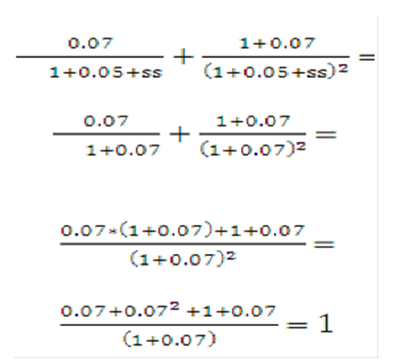
Plugging this value in the right side of the earlier equation yields:

Equation 5

Figure 10-5 Equation 5

Description of the Transfer Pricing Option Cost Equation 5 follows:

This is equal to par.

The OAS is the solution to the following equation:

Equation 6

Figure 10-6 Equation 6

Description of the Transfer Pricing Option Cost Equation 6 follows

Description of the Transfer Pricing Option Cost Equation 6 follows

By trial and error, we find a value of 1.88%. To summarize:

option cost = static spread - OAS=2%-1.88%=12 bp