11 Control & Tactical Center

Using the Control & Tactical Center, a user can access Strategy & Policy Management. This is the central place for managing the configurations of different applications and for setting up and configuring the demand forecasting runs.

In addition, a user can access the modules for managing product attributes (Attribute Extraction and Attribute Binning) as well as the link for managing web service-related credentials under the Control & Tactical Center.

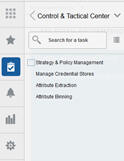
Depending on the role, a user will see one or multiple of the following links, as shown in Figure 11-1. The administrator user will have access to all of the links.

• Strategy and Policy Management

• Manage Credential Stores

• Attribute Extraction

• Attribute Binning

Figure 11-1 Control and Tactical Center

Description of "Figure 11-1 Control and Tactical Center"

Strategy & Policy Management

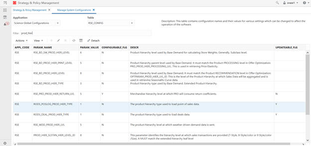
In Strategy & Policy Management, a user can edit the configurations of different applications via the Manage System Configurations functionality. In this screen, the tables can be filtered by applications.

To edit a row in any table, click the row and click the Edit icon. You can override the values for the columns that are editable.

Use the Manage Forecast Configurations to set up, manage, and configure the demand forecasting runs for different applications such as IPO-Demand Forecasting (IPO-DF), Lifecycle Pricing Optimization (LPO), IPO-Inventory Optimization (IPO-IO), Merchandise Financial Planning (MFP), and Assortment Planning (AP).

Figure 11-2 Strategy & Policy Management Dashboard

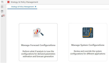
Description of "Figure 11-2 Strategy & Policy Management Dashboard"

Figure 11-3 Manage System Configurations

Description of "Figure 11-3 Manage System Configurations"

Manage Business Rules

In the Promotion Lift module, promotion data from RPM flows through RI into AIF. This enables the modeling of promotions based on the promotions the retailer has defined at the lowest level.

The following three levels in the hierarchy are used to define a promotion.

• Campaign: The highest level in the promotion hierarchy. A campaign can be used to group one or more promotions specific to an event or a holiday (for example, Fall campaign, Christmas campaign, and Back to School campaign).

• Promotion: A campaign can be further divided into smaller time frames. For example, a Christmas campaign can be divided into a Week 1 promotion, a Week 2 promotion, and a Week 3 promotion. During a promotion, multiple offers can be active.

• Offer: An offer defines the mechanism used during a promotion (for example, BOGO, 20% Off, 50% Off, TV Ad, and Gift with purchase).

The user can manage promotion data in the Data Management module to clean up the campaign and offer data.

The raw data provided by the retailer may not be suitable for the modeling of promotions. Consider, for example, information about two fall campaigns, one in 2022 and one in 2023. If the year information is present in the campaign description, it must be removed for modeling purposes as well as to estimate the lifts associated with fall campaign and to apply the observed lift values for future fall campaigns in following years. Similarly, an offer description may contain unwanted information such as month or product descriptions. After the data is cleaned up, the campaign and offer names are referred to as Campaign alias and Offer alias. These values are passed to the Promotion Lift module so that the lift values can be estimated.

The following section describes the management of promotion forecasting data. The process for estimating promotion lifts is described under Parameter Estimation.

Promotion Forecasting Data Management

Access the Data Management module from the AI Foundation Cloud Services page as follows:

Tasks -> Control and Tactical Center -> Strategy & Policy Management -> Manage Business Rules & Strategies -> Rules Category: Data Management

The Strategy & Policy Management window opens.

Figure 11-4 Strategy and Policy Management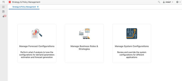

Select Manage Business Rules & Strategies. You see the Rules and Strategies Overview screen. Under Rules Category, select Data Management to view the screen for managing the campaign and offer data in AIF.

Figure 11-5 Data Management

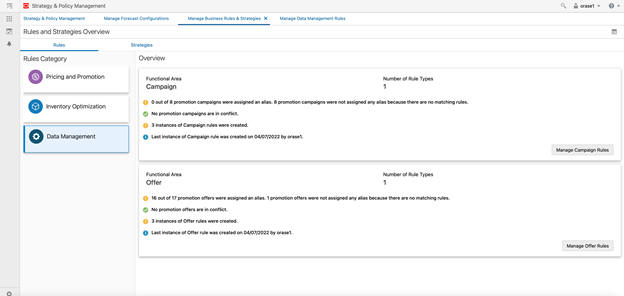
Both Campaign data and Offer data are managed in a similar way; the following process describes managing the Offer data.

Select Manage Offer Rules

When you select Manage Offer Rules, you see the following three tabs.

• Offers: This tab contains the offer data received from the retailer. Review the data to understand the various offers used and pay attention to prefixes or suffixes to the offers that do not add value or that may have an impact on the lift estimation. Similar offers can be grouped together if necessary. For example, BOGO 50% and BOGO 100% can be combined to generate BOGO.
• Rules: Rules can be created to remove unwanted descriptions from the offer data.
• Results: Review the results after the rule is applied and make changes to the rule if necessary.

The Summary panel, located below the tab, displays the following metrics.

• Number of offers: Offers received from the retailer through the data file.
• Number of offers with rules: After each rule is created, this metric is updated by the total number of offers for which an alias value is generated by a rule.
• Number of offers with conflicts: Occasionally, multiple rules can impact an offer with conflicting results. This alerts the user of the need to review the rules and make changes.

You then see multiple offers for the following.

• TV Ad with Month and Year. The month and year can be removed using rules to generate an offer alias of TV AD corresponding to these offers.
• Price Discount with Year and Season: The year and season can be removed using rules to generate an offer alias of Price Discount corresponding to these offers.
• Web Promo: Multiple offers associated with the web promotion can be grouped by creating an appropriate rule to generate an offer alias Web Promo.
• % Off: All the offers with % Off can be grouped to generate an alias % Off.

Figure 11-6 Offers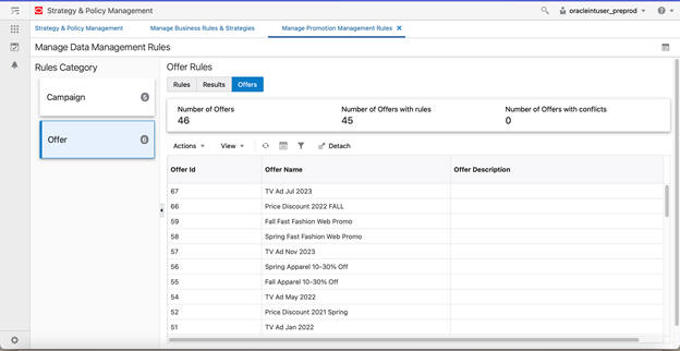

Select the Rules tab to see the following screen. This is used to create the new rules and review the existing rules. In this example, rules have already been created for Price Discount, Web Promo, and TV Ad. Select the + symbol to view the Create Rule screen. To edit a rule, select an already defined rule and click Edit.

Figure 11-7 Rules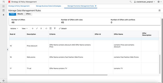

Create or Edit Offer Rules

The following must be provided for each rule.

• Description: Add a description to help manage the rules. This is used only in the Promotion Data Management screens.
• Rule criteria: Define the rule using the Query Builder. Use the Offer Name, Offer ID, and Offer Description columns to define the rules. Select one or more columns to define the rule. For each selected column, select the criteria from the drop-down menu.
• Rule value: Enter the alias value to associate with offers satisfying the rule criteria.

In the following example, all offer name that contain the % are identified and assigned a value of % Off. Click OK and save the rule. The Summary metrics are updated. You then see the Rule tab where you can review all the rules that have been created.

Figure 11-8 Query Builder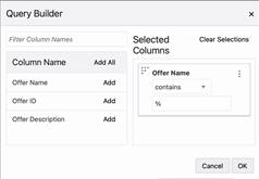

From the Rules tab, review the data for any conflicts in the Summary tab. You can select the Results tab to review the results and any conflicts.

Figure 11-9 Rules Tab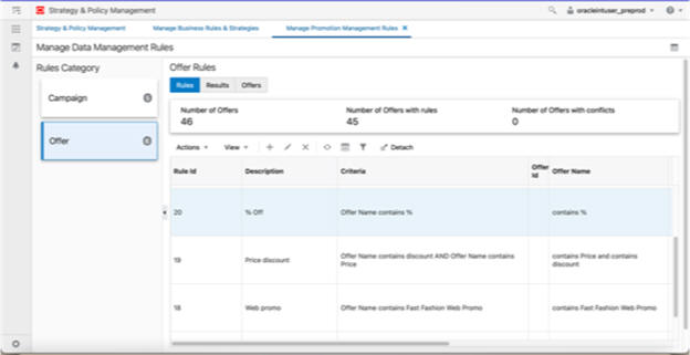

In the following Results tab, the Offer alias assigned to each Offer ID is shown. If there are conflicts for an Offer ID, a drop-down menu with multiple offer alias values associated with the Offer ID is displayed. To override the conflict, select one of the alias values in the UI or update the associated rules to remove the conflicts.

Figure 11-10 Example Results Tab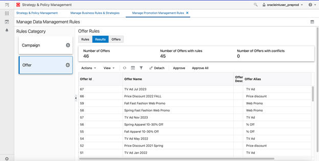

Manage Forecast Configurations

This section describes the workflow and screens in Manage Forecast Configurations. With this functionality, you can set up and manage the forecast run types and forecast runs for different applications.

You can access Manage Forecast Configurations from the Strategy & Policy Management dashboard under the Control & Tactical Center.

Forecast Run Type

The Forecast Run Type is the high-level template for forecast runs. Each run type has certain attributes that must be specified when the run type is being created. All configuration parameters default to the system default value when the run type is created. Use the Manage screen to modify the value of the configuration parameters for the run types.

Forecast Run

Forecast runs are created for a specific run type and are considered instances of the run type. The forecast run shares all the attributes of the run type and by default will have system default values for all configuration parameters. These parameters can be modified when a new run is being created in the Test screen.

Overview

The typical workflow for setting up run types, runs, and configuring the parameters is outlined in this section. Each step is described in detail in the sections that follow.

1. Create a run type in the Setup screen.

   If the aggregation status of the run type is Not Started, start the aggregation.

2. Create a run in the Test screen and override the configuration parameters as desired. Then submit the run.

3. Once the run is successfully completed, review the summary of outputs by clicking the Summary link next to the run. This feature is available only if the run uses the Causal forecast method.

   Note:

   you can create as many runs as desired. These are considered what-if runs and allow you to experiment with different values for configuration parameters and examine the impact on the estimated demand parameters.

4. Set the configuration parameters for the run type in the Manage screen. This will determine the values that should be used in all subsequent batch runs for the given run type.

   At the end of the implementation process, activate the run type to indicate that the run type should be part of the weekly batch process. During the weekly batch, a new run is created for each active run type.

5. Create a mapping between the run type and the application using the Map screen.

Setup

In the Setup screen in train stop 1, shown in Figure 11-11, you can see the overview table of the existing run types and create new run types. In addition to Run Type Name, Run Type Description, Created On, and Created By, the table shows the following information about the run type.

Figure 11-11 Run Types

Description of "Figure 11-11 Run Types"

Run Type Status

The Status column in the run type overview table shows whether the run type is Active or Inactive. Active run types become part of the weekly batch process, and a new batch run is created and executed for each active run type. Run types can be activated in the Manage screen (train stop 3).

Aggregation Status

The Aggregation Status column in the run type overview table shows whether the data aggregation for the run type is Not Started, In Progress, or Complete. Instances of runs can be generated for a run type (in the Test screen in train stop 2) only if the aggregation is complete.

Cumulative Aggregation Status

The Cumulative Aggregation Status column in the run type overview table shows whether the cumulative data aggregation for the run type is Not Started, In Progress, or Complete. Cumulative data aggregation is only applicable for run types with forecast method Causal-Short Life Cycle.

Forecast Intersection

The Forecast Intersection column in the run type overview table shows the merchandise-location-calendar intersection for which the forecast is generated. The intersection includes price zone and/or customer segment if the run type has those dimensions.

Applications

The Applications column in the run type overview table shows the application(s) that the run type is mapped to. You can map run types and applications in the Map screen in train stop 4.

External Application Key

The External Application Key column in the Run Type Overview table shows whether the external application run type key is not yet assigned to the assigned external key. You can assign the external application key for a run type (in the Map screen in train stop 4) only if the mapped application is to IPO-Demand Forecasting.

Create a Run Type

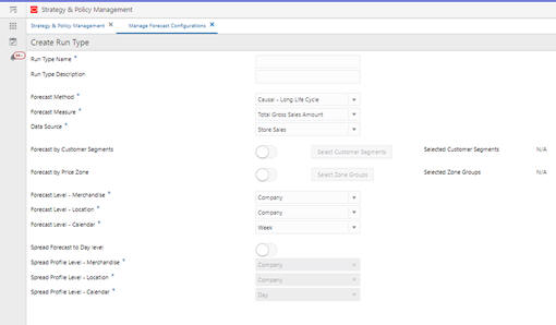
To create a new run type, click the + (plus) icon above the run type overview table. In the Create Run Type pop-up, as shown in Figure 11-12, you must specify the value for the following fields.

Figure 11-12 Create Run Type

Description of "Figure 11-12 Create Run Type"

Run Type Name

This is a unique name and must be less than 30 characters. The run type name is used as an identifier when the forecast output is exported to other applications.

Forecast Method

A forecast method must be specified for each run type. All the runs created for the run type will use the selected forecast method. The methods that are currently supported are Causal-Long Life Cycle, Causal-Short Life Cycle, and Automatic Exponential Smoothing. The forecast method must be chosen based on the specific use case and application.

Forecast Measure

This determines the measure that will be used as input by the forecasting algorithm. The final forecast will be generated for this measure. For the Causal- Short Life Cycle and Causal-Long Life Cycle methods, the supported measures are gross sales amount/unit and net sales amount/unit. For the Automatic Exponential Smoothing method, the forecast can be generated for other measures such as clearance sales and regular and promotion sales.

Data Source

This determines which data will be used as input to the selected forecast method. The source that is currently supported is the store sales and warehouse sales.

Customer Segment

Select Forecast by Customer Segments to generate the forecast by the merchandise/location/segment. If you turn on the switch, you must also click the button next to it in order to select one or multiple customer segments. It is recommended that you only select the segments that you want the forecast to be generated for (that is, un-select inactive segments) as this will make the data aggregation and forecast generation processes more efficient. Forecast by Customer Segment is applicable only for the Causal- Short Life Cycle method.

Price Zone Group

Select the Forecast by Price Zone to generate the forecast by merchandise/location/price zone. If you turn on the switch you must also click the button next to it in order to select one or multiple zone groups. It is recommended that you only select the zone groups that you want the forecast to be generated for (that is, un-select inactive zone groups) as this will make the data aggregation and forecast generation processes more efficient. Forecast by price zone is applicable only for Causal- Short Life Cycle method.

Forecast Level- Merchandise/Location/Calendar

Select the intersection that you want the forecast to be generated at. This will also determine the level at which sales data will be aggregated and flow through the various stages of forecasting. If you turn on the Forecast by Price Zone, the location level defaults to a level at the top of the location hierarchy. (This level is configurable and is determined by PMO_MIN_LOC_HIER_PROCESSING_LVL in the RSE_CONFIG table.)

Spread Profile Level — Merchandise/Location/Calendar

You can turn on the switch for the Spread Forecast to Day level only if the Forecast Level – Calendar is Week. Select the Spread Forecast Level for Merchandise/Location/Calendar only after turning on the switch for the Spread Forecast to Day level.

Data Aggregation

After you create a run type, you can see the aggregation status in the run type overview table. If the new run type has the same merchandise-location-calendar intersection as an existing run type, the aggregation status will be shown as complete as soon as you create the new run type because the data aggregation at that intersection has already been completed. This is applicable only for the run types that do not have a price zone and/or customer segment dimension. For the run types that do have a price zone and/or customer segment dimension, data aggregation must be done for each run type separately.

If any run type has an aggregation status of Not Started, click the Start Data Aggregation button above the run type overview table. This opens a pop-up where you can see a list of run types for which the aggregation process has not yet started, as shown in Figure 11–8. You can select one or multiple run types from the top and/or bottom section in the pop-up and click Submit to start data aggregation. The Cumulative Aggregation process will be started once the aggregation process is submitted. It is only applicable for run types with forecast method Causal-Short Life Cycle.

Add Multiple Run Types

Click on the Add Multiple Run Types button. It will open a tab with a table consisting of available templates to create multiple run types at a time, as shown in **INTERNAL XREF ERROR**. If the Enable column value is Y and Process Flag column is null, then the corresponding row will be considered for creating run type. Click on the Create Run Types button to create multiple run types.

Click on + icon to add new process ids to the table, as shown in **INTERNAL XREF ERROR**. Select rows from the table and click on X icon to delete process ids. User can also edit parameters within each row if Process Flag is null. Click on Save button to save the changes.

Figure 11-13 Add Multiple Run Types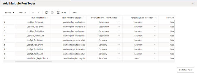

Figure 11-14 Specify Run Type Configurations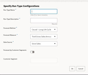

Delete Run Type

Select one or multiple rows in the run type overview table, as shown in **INTERNAL XREF ERROR**, and click the X icon above the table to delete the run types. If a run type is activated or if a run type has a run that is in progress, it cannot be deleted.

Figure 11-15 Select Aggregation Levels and Run Types

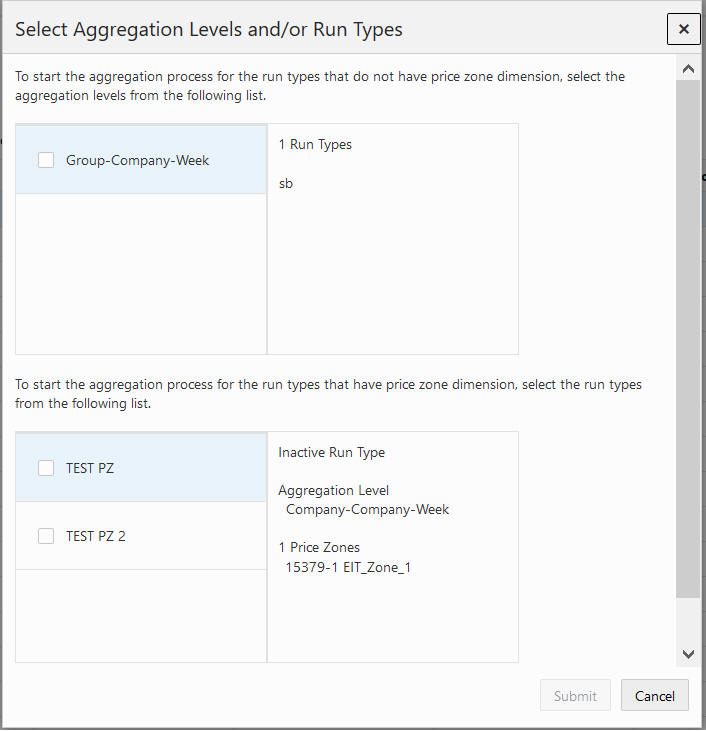
Description of "Figure 11-15 Select Aggregation Levels and Run Types"

Test

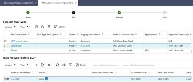
After the run types are created and aggregation is complete, you can create and submit what-if runs and review the summary of the runs in the Test screen in train stop 2, as shown in Figure 11-16. Performing what-if analysis is an optional step that can help you to tune the various configuration parameters. In addition, you can see the batch runs associated with each run type in this screen.

Figure 11-16 Test Screen

Description of "Figure 11-16 Test Screen"

In the Test screen, the top table shows all the run types that have complete aggregation. This table shows the same information as the run type table in the Setup screen. The bottom table shows all the what-if runs and batch runs associated with the selected run type in the top table. In addition to Run Name, Created On, Created By and Complete On, the table shows the following information about the run.

Run Status

The Status column in the run overview table shows the progress of the run by showing the status of the different stages of estimation and forecasting.

• Setup

• Preprocessing in Progress, Preprocessing Failed

• Preprocessing Complete - Estimation in Progress, Preprocessing Complete - Estimation Failed

• Estimation Complete - Base Demand in Progress, Estimation Complete - Base Demand Failed, Estimation Complete - Base Demand Complete, Estimation Complete - Base Demand Complete with Zero Rows

• Estimation Complete - Forecast Generation in Progress, Estimation Complete - Forecast Generation Failed, Estimation Complete - Forecast Generation Complete, Estimation Complete - Forecast Generation Complete with Zero Rows

Estimation Run

In all forecast methods, the estimation process runs initially to generate the demand parameters such as seasonality and elasticity. Subsequently, the forecast process runs to generate the base demand and the forecast using the outputs from the estimation process. The Estimation Run column shows the name of the estimation run that is behind the forecast run:

Run Type Name

Each run is associated with a run type. This column shows the name of the run type.

Results

This column shows the link to different output screens. The Summary link opens a tab that provides information about the different stages of demand parameter estimation. This link is enabled for all Causal-Short Life Cycle runs for which the estimation process has completed successfully.

Create What-If Run

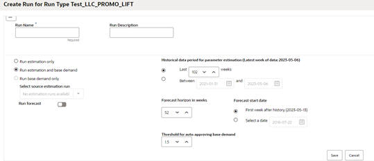
To create a what-if run, first select a run type by selecting a row in the top table. Then, click the + (plus) icon in the bottom table to open the Create Run pop-up, as shown in Figure 11-17.

Figure 11-17 Create a Run

Description of "Figure 11-17 Create a Run"

The menu on the left shows the different stages of estimation and forecasting. These stages can be different, depending on the forecast method that was selected for the run type.

You can set the scope of the run, the run name, and the description in the first tab. In the left side of the Scope tab, select Run Estimation Only to execute the end-to-end process for estimating demand parameters. Select Run Estimation and Base Demand to execute the end-to-end process for estimating demand parameters and generating base demand. Alternatively, you can select Run Base Demand Only and then select an estimation run from the list of previously completed estimation runs. If no such run exists, this option will be disabled. If the completed estimation run is selected, then the historical data period section will be populated based on the run and will be disabled. To also generate the forecast, turn on Run Forecast. Forecast generation for a price zone run type will always be disabled.

In the right side of the Scope screen, you can select the period of historical data that should be included in the estimation process. This part will be enabled only if Run estimation and base demand is selected. You can either select a period by specifying the start and end date or by specifying the number of weeks to be used from historical data. In the Scope tab, you can also specify the time period for the forecast generation by selecting a start date for forecast period and a forecast horizon. You can also set the threshold used for auto-approving base demand. The base demand values that are less than this threshold times the average rate of historical sales are approved.

In the other tabs on the left menu, you can review and override the configuration parameters for each stage of the estimation and the base demand/forecast. To override a parameter, select the row in the table and click the Edit icon above the table. For the Elasticity and Seasonality tabs, you can override the parameters at different levels of merchandise and location, as shown in the following figure. This feature is applicable only for the Causal-Short Life Cycle and the Causal-Long Life Cycle run types. For other tabs, parameters can be overridden only at global level. The levels that are valid for the override depends on the stage, that is, for elasticity and seasonality this is closely tied to escalation levels.

You can click the Add a parameter override button to override parameters at different levels of merchandise and location, as shown in the first of the following three figures. The Active flag allows the user to not use an override temporarily without having to delete it. Once the parameter is overridden at selected intersection, you can add the override at multiple intersections by clicking Save and add another button. This override display in the table is shown in the second of the following three figures. The Base Demand tab override can be performed in three ways: at the global level, at a single merchandise-location parent level, and at the base demand level, which is essentially the aggregation level of the run, as shown in the third of the following three figures.

Figure 11-18 Override Parameters at the Intersection for Elasticity/Seasonality

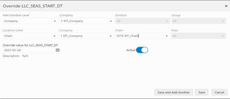
Figure 11-19 Override Parameters Table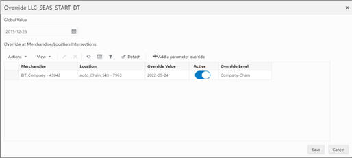

Figure 11-20 Override Parameters at the Intersection for Base Demand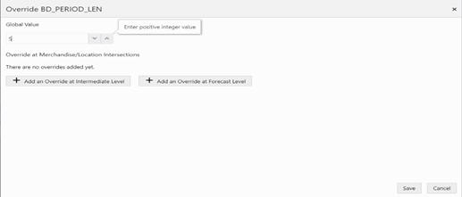

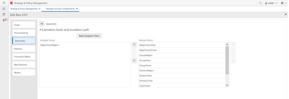
In the Seasonality tab, in addition to the configuration parameters, you can also modify the escalation path by selecting or unselecting the merchandise-location intersections that will be used during escalation process.

For the Causal-Long Life Cycle runs in the Promotion Effects tab, you can edit the configuration parameters and Algorithm, Partition and Reliability Metrics, as shown in the following figure.

In the Review tab, you can see all the parameters that were overridden and submit the run for the execution.

Figure 11-21 Edit Promotion Effects for LLC Run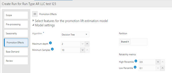

For details about different configurations parameters for Causal-Short Life Cycle runs, see the Oracle Retail AI Foundation Cloud Services Implementation Guide.

Figure 11-22 Edit Run

Description of "Figure 11-22 Edit Run"

Duplicate Run

Select a row and click the Duplicate icon above the table to create a copy of an existing run. The run will be created in Setup status.

Delete Run

Select one or multiple rows and click the X icon above the table to delete a run or runs. If a run is in progress, it cannot be deleted. For each run selected to be deleted, you see three options: Cancel, Delete Forecast Run and Delete Forecast and Estimation Run. The Delete Forecast Run button deletes the forecast run. The Delete Forecast and Estimation Run button deletes the forecast run and in addition deletes the estimation run that is behind the forecast run. You can perform the Delete Forecast and Estimation Run only when there is no other forecast run tied with same estimation run. For the Automatic Exponential Smoothing run type, only the Delete Forecast and Estimation Run can be performed, as each forecast run is mapped with a different estimation run.

Approve Demand Parameters

Select a row and click the Approve Demand Parameters button above the table to approve the estimation runs. You can approve demand parameters only for the runs where the estimation is complete. You can approve another run to replace the previously approved run. Once a run is approved, the Estimation Run column in the below table displays Approved next to the estimation run name. The demand parameters generated by the approved run will be used in weekly forecast batch runs.

Approve Base Demand and Forecast

Select a row and click the Approve Demand and Forecast Parameters button above the table to approve base demand and forecast runs. Approve Base Demand and Forecast operation can be performed for the runs that has an approved estimation run. Once a run is approved, the Forecast Run Name column in the below table displays Approved besides the forecast run name.

Manage

In the Manage screen in train stop 3 you can set the value of configuration parameters for the run type. These values will be used when creating and executing batch runs for each run type. In this screen, you can also activate or inactivate run types by selecting a row and clicking the Activate button above the table. Active run types become part of the weekly batch process, and a new batch run is created and executed for each active run type. For each active run type, once the batch run is approved, the output of the batch run will be exported to and consumed by the applications that are mapped to that run type. In order to auto-approve the batch runs, select a row and click on Manage Auto-approve. For the Causal-Short Life Cycle run type, the start date calculation can be disabled or enabled by clicking the Disable Life Cycle Start Date Calculation/ Enable Life Cycle Start Date Calculation button, respectively.

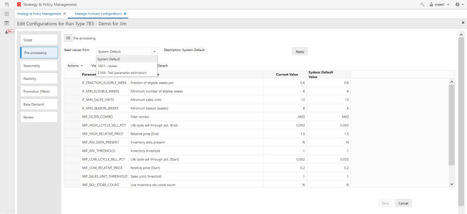
To review and override the value of configuration parameters for a run type, select a row and click Edit Configuration Parameters above the table. This button will be disabled if the run type is in active status. The Edit configuration pop-up is similar to the Create Run pop-up that is used to create forecast runs and has a tab for each stage of estimation and forecast. In each tab, you can do one of the following, as shown in Figure 11-23.

• Set the values of all configuration parameters in that stage, based on the system default for the run type. To do this, select System Default from the drop-down menu and click Apply.

• Set the values of all configuration parameters in that stage based on the values that were previously set in one of the what-if runs. To do this, select the desired run from the drop-down menu and click Apply.

• Override the value of a certain configuration parameter. To do this, select a row and click the Edit icon above the table.

Figure 11-23 Edit Run Type Configuration

Description of "Figure 11-23 Edit Run Type Configuration"

Promotion Effects

In the Promotion Lift module, promotion data from Pricing CS or other sources flows through RI into AIF. This enables the modeling of promotions based on the promotions defined by the retailer at the lowest level. The following three-level hierarchy is used for defining the promotions.

• Campaign: The highest level in the promotion hierarchy. A campaign can be used to group one or more promotions specific to an event or holiday (for example, Fall Campaign, Christmas campaign, or Back to School campaign).
• Promotion: A campaign can be further divided into smaller time frames. For example, a Christmas campaign can be divided into a Week 1 Promotion, Week 2 Promotion, and Week 3 Promotion. During a promotion, multiple offers can be active.
• Offer: An offer defines the mechanism used during a promotion (for example, BOGO, 20% Off, 50% Off, TV Ad, or Gift with purchase).

The user can manage promotion data from Manage Business Rules & Strategies in the Data Management section to clean up the campaign and offer data.

The raw data provided by the retailer may not be suitable for the modeling of promotions. Consider for example information about two fall campaigns, one in 2022 and one in 2023. If the year information is present in the campaign description, it must be removed for modeling purposes as well as to estimate the lifts associated with fall campaign and to apply the observed lift values for future fall campaigns in following years. Similarly, an offer description may contain unwanted information such as month or product descriptions. After the data is cleaned up, the campaign and offer names are referred to as Campaign alias and Offer alias. These values are passed to the Promotion Lift module so that the lift values can be estimated.

This section describes the process for estimating promotion lifts. As part of promotion effects, select the following.

• Features used by the model to determine the promotion lift values.
• Promotion model settings.

Forecast Configuration — Promotion Features

Select the Promotion Effects tab corresponding to a parameter estimation run to view the following.

• Select features for the promotion lift estimation model.
• Model settings.

The following screen shows the various features that are available to the user. These various features can be classified according to the following categories.

• Promotion related: Campaign Name, Offer Name, Campaign Description, Offer Type, and Offer Description.

  • Campaign Name and Offer Name contain the campaign alias and offer alias values that are assigned through the data management module; these are always selected.

  • In addition to the alias values, one or more of the following features can be enabled if they are useful: Campaign Description, Offer Description, and Offer Type. Review the data to decide which of these features will be useful.

• Product Hierarchy: Promotion feature product hierarchy

  • Multiple levels of the product hierarchy can be selected as features to the model (for example, Class and Department). This allows the model to search for variations at each of the selected levels.

• Location Hierarchy: Promotion feature location hierarchy

  • Multiple levels of location hierarchy can be selected as features to the model (for example, Area and Region). This allows the model to search for variations at each of the selected levels.

• Product Attributes

  • Two attributes are supported. Select the relevant attributes that impact the promotion lift.

• Location Attributes

  • Two attributes are supported. Select the relevant attributes that impact the promotion lift.

• Performance Metrics: % sales on promotion, % Weeks on promotion

  • In addition to the hierarchy and attributes, products can behave differently. Some products might be highly promotional compared to others. These features can be used to capture the variation lifts observed for different types of products, as determined by each performance metric.

Figure 11-24 Promotion Effect Forecast Configuration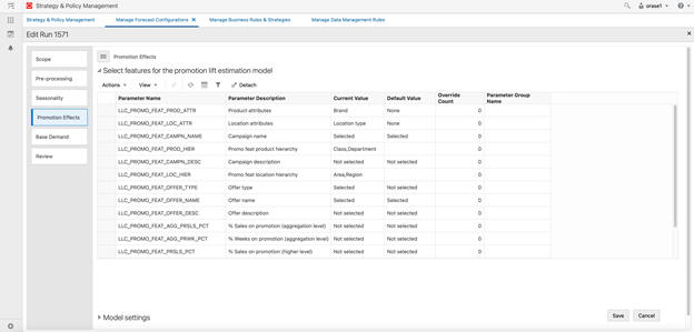

For a given retailer, start with a small selection of features that you expect to have an impact on promotion lifts and add new features to see if the addition of the feature improves the model performance. The details for reviewing the model output are provided after the model settings.

Model Settings

Algorithm: Select Decision tree. GLM is also available.

Minimum samples: Minimum number of data points for each leaf node of the decision tree. This is used to ensure there are enough data points for each node.

Maximum depth: Number of levels between the leaf node and the top of the decision tree. Start with a value between 4 and 6, depending on the number of features being used and increase the number gradually to see if the model performance improves.

Partition: The model can be partitioned, based on one or more of the features used for building the model. Selecting a partition builds a separate model for each value corresponding to the chosen partition. Multiple features can be selected to determine a partition. Partitioning by higher levels in the product hierarchy and the location hierarchy or based on relevant product/location attributes can help to determine the promotions lifts more accurately. Lower levels of product/location hierarchy may not have sufficient data to create reliable parameters.

Reliability metrics:

High percentile: A value of 0.9 removes the top 10 percent of the observed lift values for building the model. Adjust the setting to remove outlier values with very high lift.

Low percentile: A value of 0.1 remove the bottom 10 percent of the observed lift values for building the model. Adjust the setting to remove outlier values with very low lift.

Figure 11-25 Promotion Effects Output Review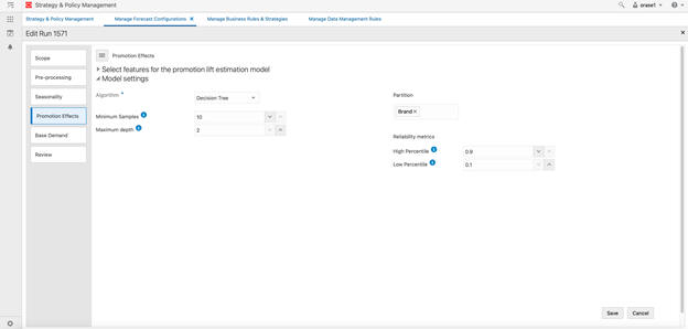

Review the output of the promotion effects:

• Pmo_llc_pl_model: Contains the details about the promotion model.
• Case table, Case columns: Contains all the features available for the user to select.
• View name, View columns: Based on the user selection in the UI.
• Using IW, Model name can be used to apply the model for a chosen time frame on the case table.
• RMSE and MAE: Error in lift value.
• Avg_error, Median error and Error_Wgt: % Error.
• Error_wgt: % Error weighted by sales units.

Figure 11-26 Promotion Effects Output

Map

In the Map screen in train stop 4, you can map run types to applications. There can be many-to-many mappings between the run types and applications. For example, if Lifecycle Pricing Optimization requires a forecast of two different measures (for example, total net sales quantity and total net sales amount), there will be two run types and both must be mapped to Lifecycle Pricing Optimization. Also, if two different applications (for example, Lifecycle Pricing Optimization and Inventory Planning Optimization-Inventory Optimization) both require a forecast for the same measure and at same intersection, the two application will be mapped to the same run type.

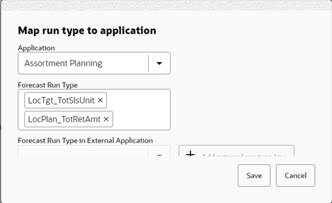
You can select more than one run type at a time to be mapped to an application other than IPO-DF, as shown in **INTERNAL XREF ERROR**.

You can assign an external application key to run the types in this section. An external application run type key value can only be assigned to a run type when the selected application is IPO-DF. Two run types that have the exact same prod/loc/cal/forecast measure/data source but opposite life cycles can have the same external application run type key. Basically, for each external application run type key, there can be at most one run type from each life cycle, so at most one Causal-Long Life Cycle run type and at most one Causal-Short Life Cycle run type, and those two run types must have the same prod/loc/cal/forecast measure/data source.

To create a new mapping, click on the + (plus) icon above the table in Map screen. Select an application and a run type from the drop-down menu and click Save. To delete a mapping, select a row and click the X icon above the table.

Figure 11-27 Map Run Type

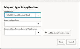
Figure 11-28 Providing Additional Map Run Type

Manage Master Data

You can access Manage Master Data from left side Tasks list as shown in the following figure.

Figure 11-29 Manage Master Data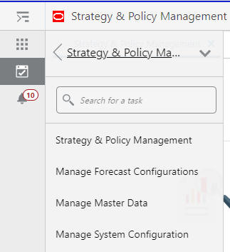

In Sales Plans tab, as shown in the following figure, you can select a row and edit the Merchandise Level/Location Level or reset the value to the default levels.

Figure 11-30 Sales Plan

In the Flexible Groups tab, the Flexible Groups provides for grouping sku/stores based on different criteria. Group Set is the parent (that is, the grouping definition). Partitions are the children (that is, the groups within each group set). As shown in the following figure, you can create a new flexible group set and edit and delete an existing flexible group set. While creating a new flexible group set, you can add a new name (which must be unique), description, and select a run type name from the drop-down list, as shown in the following figure. However, the partitions are provided through the interface. By clicking the icon near group set name, you can see the partitions under it.

Figure 11-31 Flexible Groups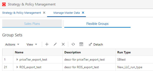

Figure 11-32 Create Flexible Group Set

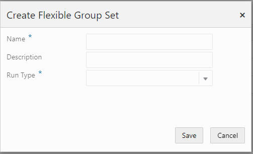
Figure 11-33 Partitions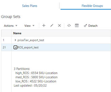

Once a new flex group set is created, a new entry corresponding to the flex group set will be added to the Available Values section of Estimation Levels and Escalation Path of Seasonality tab in Edit Configuration Parameters, as shown in the following figure.

Figure 11-34 Edit Configurations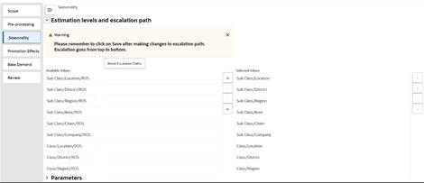

When a new What-If run is created under the corresponding run type, the run will also contain the addition escalation levels corresponding to the flex group set and will be displayed in the Available Values section.

Manage Credential Stores

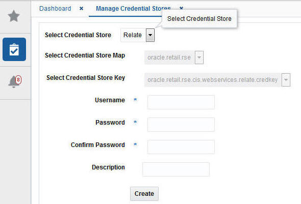
Oracle Customer Engagement web service-related credentials are managed in the credential stores using the interface shown in Figure 11-35. The administrator can use this screen to configure the name and password. This information is used to generate the authentication key that is sent as part of the message to Oracle Customer Engagement.

Figure 11-35 Manage Credential Stores

Description of "Figure 11-35 Manage Credential Stores"

The Credential Stores dialog box requires the following information:

• Label - describes the credential store map and key

• Username - user name provided by Oracle Customer Engagement

• Password - password provided by Oracle Customer Engagement

• Confirm Password - prompt to confirm user password

• Description - used by the administrator to describe the credential store used for Customer Segment integration with Oracle Customer Engagement.

Attribute Extraction and Attribute Binning

For details about the screens of Attribute Extraction, refer to Attribute Extraction.