7 Working with Spark
This chapter describes the various concepts involved in working with Spark.
This chapter includes the following sections:
Spark Usage
To use Spark engines, a Staging Execution Unit must be created in the Physical Mapping and the EU execution location must be set to Spark Schema.
Creating a Spark Mapping
Pre-requisites for handling Avro and Delimited files in Spark Mappings
Avro files
For using Avro files in Spark mappings, the Avro .egg file has to be added to the ODI installation. The .egg file for Avro cannot be downloaded directly, and has to be generated from the Avro package.
To add the Avro .egg file to the ODI installation:
-
Generate the .egg file from the Avro Package
-
Download
avro-1.8.0.tar.gzfrom avro 1.8.2 : Python Package Index or Apache Avro™ Releases. -
Unzip it, and install the Avro Python library as shown below.
$ tar xvf avro-1.8.1.tar.gz
$ cd avro-1.8.1
$ sudo python setup.py install
Installed /usr/lib/python2.6/site-packages/avro-_AVRO_VERSION_-py2.6.egg
Processing dependencies for avro===-AVRO-VERSION-
Finished processing dependencies for avro===-AVRO-VERSION-
The
avro-_AVRO_VERSION_-py2.6.eggfile can now be found in the Python installed directory.For more information, see Apache Avro™ 1.8.0 Getting Started (Python).
-
-
Copy the
.eggfile to a specific location in ODIFor ODI Agent, copy the
.eggfile to$DOMAIN_HOME_PROPERTY/lib/spark.For ODI Studio, copy the
.eggfile to$HOME/.odi/oracledi/userlib/spark.
Delimited files
For using Delimited files in Spark mappings, external jar files must be added to the ODI installation.
To add the CSV jar files to the ODI installation:
-
Download the CSV jar files
Download the following jar files from their corresponding links:
-
spark-csv_2.10-1.5.0.jarfrom spark-csv -
commons-csv-1.2.jarfrom Commons CSV – Download Apache Commons CSV
-
-
Copy the jar file to a specific location in ODI
For ODI Agent, copy the jar files to
$DOMAIN_HOME_PROPERTY/lib/spark.For ODI Studio, copy the jar files to
$HOME/.odi/oracledi/userlib/spark.
Spark Design Considerations
If you have chosen to use Spark as your Transformation Engine, you must take the following design decisions before writing your Mappings:
Batch or Streaming
Spark supports two modes of operation — Batch and Streaming. In Streaming mode, you can ingest data from Kafka Topics, or Files/HDFS Files added to a specified location. To get the most out of Streaming, see Spark Checkpointing and Spark Windowing and Stateful Aggregation.
To set the Streaming flag, select Physical Design, click the blank canvas, and select the Streaming checkbox on the property panel. If the Streaming flag is not set, the mappings will execute in Batch mode (default).
Resilient Distributed Datasets (RDD) or DataFrames
Spark has more than one set of APIs that can be used to transform data. Resilient Distributed Datasets (RDD) and DataFrames are APIs that ODI can generate code for.
Resilient Distributed Datasets (RDD)
RDDs are the primary data abstraction in Apache Spark. They are fault tolerant (Resilient) collections of partitioned data (Dataset) with data residing on multiple nodes in a cluster (Distributed). The data resides in memory and is cached where necessary. RDDs are read-only, but can have transformations applied that will create other RDDs. Lazy evaluation is used, where the data is only available or transformed when triggered. RDD partitions are the unit of parallelism.
DataFrames
A DataFrame is a read-only distributed collection of data, that (unlike RDDs) is organized into named columns. The abstraction level is higher, making the processing of large datasets even easier, such as in allowing the use of SparkSQL queries. DataFrames are built on top of the Spark SQL engine, allowing for much better performance and space optimization.
Note:
If Streaming is used, RDD is the only option available.Infer Schema Knowledge Module Option
Spark can infer or deduce the Schema of a dataset by looking at the data. Although this can be advantageous, there are some circumstances where datatypes may not be mapped as expected. If this happens, there is an inferSchema option on applicable Spark KMs that can be set to False, turning off this functionality. If you see runtime errors related to datatype mismatches, you may need to adjust the value of the Infer Schema option. This option can be set on reading or writing LKMs.
Note:
Spark uses this option only while creating DataFrames. If inferSchema is set to False, ODI will generate a schema definition based on mapping data store metadata and this structure will be used to create DataFrame API.The Infer Schema option can be seen in the figure below.
Figure 7-1 Physical Mapping with InferSchema KM Option

Description of "Figure 7-1 Physical Mapping with InferSchema KM Option"
Expression Syntax
When you need to write expressions, for example, in a Join or Filter condition, or an Attribute expression, you have options that can be used for the Expression Syntax. If you have decided to have ODI generate RDD code, then your expressions must be written in Python. If, however, you have decided to generate DataFrames, then you can choose to write your expressions in SQL or Python. You can specify your chosen syntax by setting SQL_EXPRESSIONS to True/False.
The combinations of possible code generation style are:
-
RDD with Python expressions
-
DataFrames with Python expressions
-
DataFrames with SQL expressions
Since Python expressions are defined differently in RDD and DataFrames, the Python syntax for these two styles of code generation can be different. Therefore, not all Python expressions will work for both RDD and DataFrame code generation styles.
RDD with Python expressions
For information on the syntax and functions that can be used in Python expressions, see The Python Standard Library.
DataFrames with Python expressions
For information on the list of Python functions available to Column objects, see Pyspark.sql.module.
DataFrames with SQL expressions
The generic SQL functions and operators can be viewed in the Expression editor on selecting generic SQL language.
Mapping Description
Consider an example that shows multiple expressions being used in mappings.
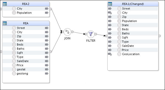
In this example, a source (REA) containing Real Estate Transactions is combined with a second source (REA2) containing City and Population data. A filter is then applied to select only large transactions. This creates a target file (REA1) which contains the combined and filtered information as shown in the figure below.
Figure 7-2 Mapping with Multiple Expressions

Description of "Figure 7-2 Mapping with Multiple Expressions"
Mapping Definitions
The mapping is defined as follows:
-
JOIN: Joins the Real Estate Transaction Table (
REA) with the City Population table (REA2) using City as the Key. The City names inREA1are in uppercase, whereas inREA2they are in lowercase. -
FILTER: Selects rows that have a price greater or equal to $500,000, and ignores transactions where Type is Multi-Family.
-
City: City names should be in lowercase except for the first letter of each word.
-
GeoLocation: This should be in the form "<longitude>, <latitude>". The quotes should be included in the string.
-
Population: Rounds off to the nearest thousand.
Mapping Expressions for each Codegen Style
The following table describes the mapping expressions for each codegen style.
Table 7-1 Mapping Expressions for each Codegen Style
| Mapping Expression for the Codegen Style | RDD with Python Expressions | DataFrames with Python Expressions | DataFrames with SQL Expressions |
|---|---|---|---|
|
Join Condition |
REA.City == (REA2.City).upper() |
REA.City == upper(REA2.City) |
REA.City = UPPER(REA2.City) |
|
Filter Syntax |
REA.Type<>'Multi-Family' and REA.Price >=500000 |
REA.Type<>'Multi-Family' and REA.Price >=500000 |
REA.Type<>'Multi-Family' and REA.Price >=500000 |
|
Target Column Syntax |
# City - note: this only capitalizes the first word! (REA.City).capitalize() # GeoLocation REA.geolat + ", " + REA.geolong # Population int(round(REA2.Population,-3)) |
# City
initcap(lower(REA.City))
# GeoLocation
concat(REA.geolat ,lit(", "),REA.geolong)
# Population
round(REA2.Population,-3) |
-- City INITCAP(LOWER(REA.City)) -- GeoLocation CONCAT(REA.geolat,', ', REA.geolong) # Population ROUND(REA2.Population,-3) |
Importing Libraries
As you'll see from this example, not all the same built-in functions are available across these differing styles. In this case, the initcap built-in function is not available in RDD. The capwords() function does what is required, but it requires import statements to be added to the script. The Spark EKM has a multi line option called customPythonImports that lets you specify the Import Statements for the script, thereby allowing extra functions to be available in the expressions.
To contain the list of imports, the customPythonImports EKM option will be written as
from string import *
from time import localtime
The Target Column expression would then be written as
#City
capwords(REA.City)
Spark Streaming Support
This section provides information about streaming modes of operation on data sets. It also provides information on Checkpointing.
This section includes the following sub-sections:
Spark Checkpointing
A streaming application must operate 24/7 and hence should be resilient to failures. Spark Streaming needs to checkpoint information to a fault tolerant storage system so that it can recover from failures.
Checkpointing is enabled for applications recovering from failures of the driver running the application. Checkpointing only ensures that the Spark application will restart from where it left if a checkpoint is found.
For additional information on checkpointing, refer to Spark Streaming Programming Guide.
Spark Windowing and Stateful Aggregation
Spark's Windowing feature allows aggregation (and other transformations) to be applied not just to the current RDD, but also include data from several previous RDDs (window duration).
The Spark KMs support batch and, also streaming transformations. While the Python code for non-streaming operates on RDD or DataFrame objects, the streaming code works on DStream objects. Aggregation in batch mode is simple: there is a single set of input records (RDD), which are aggregated to form the output data, which is then written into some target. In streaming mode the continuously incoming data is discretized into a flow of RDDs. By default each RDD is aggregated independently.
Spark windowing works well for calculating things like running sum or running averages. But it comes with two restrictions:
-
Older RDDs must be retained
-
Data falling into the window is recalculated for every new RDD.
This is the reason why windowing is not suitable for aggregation across an entire data stream. This can only be achieved by stateful aggregation.
Windowing enabled KMs have the following optional KM Options:
-
Window Duration: Duration of window defined in number of batch intervals.
-
Sliding Interval: Interval at which the window operation is performed defined in number of batch intervals.
Windowing is supported by:
-
XKM Spark Aggregation
-
XKM Spark Join
-
XKM Spark Set
-
XKM Spark Distinct
For additional information, refer to Spark Streaming Programming Guide.
Stateful Aggregation
When data must be aggregated across all data of a stream, stateful aggregation is required. In stateful aggregation Spark builds called state stream containing the aggregated values for all keys. For every incoming RDD this state is updated, for example aggregated sums are updated based on new incoming data.
By default a state stream will output all stored values for every incoming RDD. This is useful in case the stream output is a file and the file is expected to always hold the entire set of aggregate values.
Stateful processing is supported by:
-
XKM Spark Aggregate
-
XKM Spark Lookup
Spark Repartitioning and Caching
Caching
In ODI, the Spark caching mechanism is leveraged by providing two additional Spark base KM options.
-
Cache data: If this option set to true a storage invocation is added to the generated pyspark code of the component.
-
Cache storage level: This option is hidden if cache data is set to false.
Repartitioning
If the source is a HDFS file, the number of partitions is initially determined by the data block of the source HDFS system. The platform resource is not fully used if the platform that runs the Spark application has more available slots for running tasks than the number of partitions loaded. In such cases, the RDD.repartition() api can be used to change the number of partitions.
Repartitioning can be done in any step of the whole process, even immediately after data is loaded from source or after processing the filter component. ODI has Spark base KM options which let you decide whether and where to do repartitioning.
-
Repartition: If this option is set to true, repartition is applied after the transformation of component.
-
Level of Parallelism: Number of partitions and the default is 0. When the default value is set, spark.default.parallelism will be used to invoke the repartition() function.
-
Sort Partitions: If this option is set to true, partitions are sorted by key and the key is defined by a Lambda function.
-
Partitions Sort Order: Ascending or descending. Default is ascending.
-
Partition Keys: User defined partition keys represented as a comma separated column list.
-
Partition Function: User defined partition Lambda function. Default value is a pyspark defined hash function
portable_hash, which simply computes a hash base on the entire RDD row.
Configuring Streaming Support
Configuring Streaming Support is performed in two parts:
- Topology
- Mapping Design
Spark Streaming DataServer Properties
Provides the Spark Technology-specific streaming properties that are default for the Spark Execution Unit properties.
Table 7-2 Spark Streaming DataServer Properties
| Key | Value |
|---|---|
| spark.checkpointingBaseDir | This property defines the base directory for checkpointing. Every mapping under this base directory will create a sub-directory.
Example: hdfs://cluster-ns1/user/oracle/spark/checkpoints |
| spark.checkpointingInterval | Displays the time in seconds |
| spark.restartFromCheckpoint |
|
| spark.batchDuration | Displays the duration in seconds of a streaming interval. |
| spark.rememberDuration | Displays the time in seconds and sets the Spark Streaming context to remember RDDs for this duration. |
| spark.checkpointing | Enables Spark checkpointing. |
| spark.streaming.timeout | Displays the timeout in seconds before stopping a Streaming application.
Default is 60. |
| odi-execution-mode |
|
| spark.ui.enabled | Enables the Spark Live REST API.
Note: Set to true for asynchronous execution. |
| spark.eventLog.enabled | Enables Spark event logs. This allows the logs to be accessible by the Spark History Server.
Note: Set to true for asynchronous execution. |
| principal | Kerberized User name. |
| keytab | The location of the keytab file that contains pairs of kerberos principal and encrypted keys.
Example: /tmp/oracle.keytab |
| odi.spark.enableUnsupportedSparkModes | This check is introduced, as only yarn-client and yarn-cluster are supported. |
Extra Spark Streaming Data Properties
Provides the extra spark streaming properties that are specific to Spark technology that are added to the asynchronous Spark execution unit.
Table 7-3 Extra Spark Streaming Properties
| Key | Value |
|---|---|
| spark-webui-startup-polling-retries | Maximum number of retries while waiting for the Spark WebUI to come-up. |
| spark-webui-startup-polling-interval | Displays the time in seconds between retries. |
| spark-webui-startup-polling-persist-after-retries | |
| spark-webui-rest-timeout | Timeout in second used for REST calls on Spark WebUI. |
| spark-webui-polling-interval | Time in seconds between two polls on the Spark WebUI. |
| spark-webui-polling-persist-after-retries | |
| spark-history-server-rest-timeout | Timeout in seconds used for REST calls on Spark History Server. |
| spark-history-server-polling-retries | Maximum number of retries while waiting for the Spark History Server to make the Spark Event Logs available. |
| spark-history-server-polling-interval | Time in seconds between retries. |
| spark-history-server-polling-persist-after-retries | |
| spark-submit-shutdown-polling-retries | Maximum number of retries while waiting for the spark-submit OS process to complete. |
| spark-submit-shutdown-polling-interval | Time in seconds between retries. |
| spark-submit-shutdown-polling-persist-after-retries |
Switching between RDD and DataFrames in ODI
You can switch between generating DataFrame code and RDD code by setting the EKM option spark.useDataFrames to either True or False on the Spark Execution Unit.
Components that do not support DataFrame Code Generation
Some components do not support DataFrame code generation. If even a single mapping component does not support DataFrames, a validation error is shown (asking you to set the Spark Execution Unit property spark.useDataFrames to false) and you will need to switch back to RDD.
The following components do not support DataFrame code generation:
-
Pivot
-
Unpivot
-
Input Signature
-
Output Signature
Adding Customized Code in the form of a Table Function
The TableFunction component allows you to add your own code segment into the mapping in the form of a reference to an external script, or some inline code.
Consider an example where the TABLEFUNCTION component is utilized to parse and transform a source log file. The mapping will produce a target file with data as-is from the source file, modified data, and new data such as timestamps.
To build the mapping containing a table function and add input and output attributes to it, follow the below procedure:
-
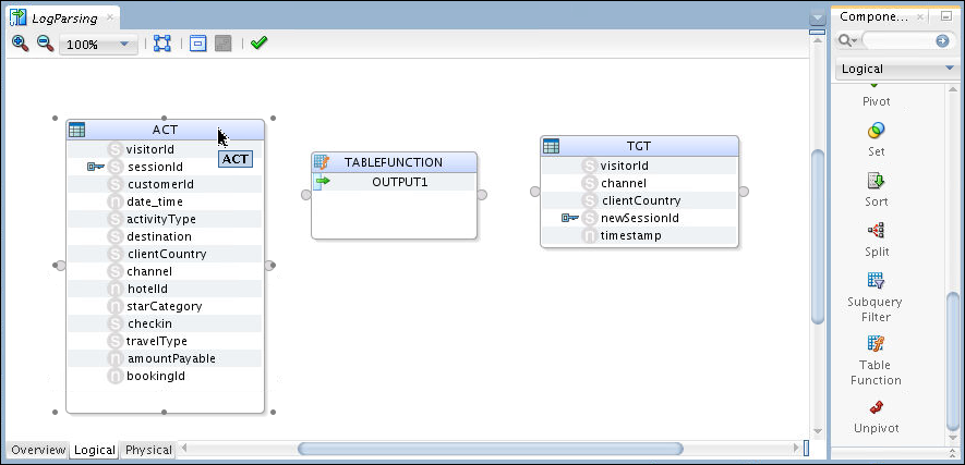
Create a mapping by adding the source and target data stores along with a table function component named 'TABLEFUNCTION'.
Figure 7-3 Mapping with Source, Target, and Table Function

Description of "Figure 7-3 Mapping with Source, Target, and Table Function" -
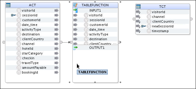
Connect the source data store’s output connector to the input connector of the TABLEFUNCTION component.
Input attributes will now be added directly to TABLEFUNCTION.
Note:
-
An input group 'INPUT1' is created automatically containing all the attributes from the source data store as shown in the figure below.
-
For each additional source data store, a new input group will be added.
Figure 7-4 Input Group added to TABLEFUNCTION

Description of "Figure 7-4 Input Group added to TABLEFUNCTION" -
-
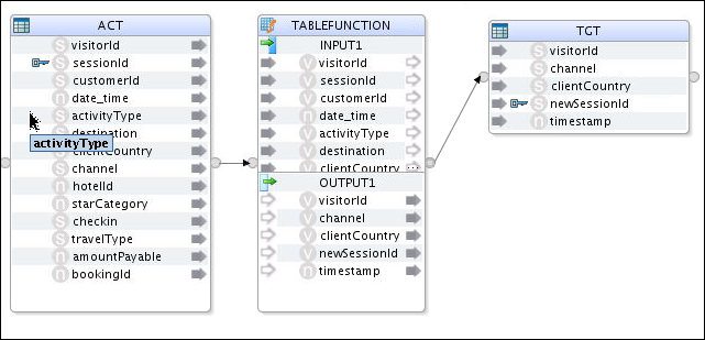
Connect the target data store’s input connector to the output connector of the TABLEFUNCTION component.
Output attributes will now be added directly to TABLEFUNCTION.
Note:
-
An output group 'OUTPUT1' is created automatically containing all the attributes from the target data store as shown in the figure below.
-
The output attributes in 'OUTPUT1' can be renamed or deleted.
-
The expression for each output attribute will be set grammatically by the script embedded in the TABLEFUNCTION component and doesn’t need to be set individually.
Figure 7-5 Mapping with Source, Target, and Table Function connected

Description of "Figure 7-5 Mapping with Source, Target, and Table Function connected" -
Configure the mapping by following the procedure below:
-
Go to the Logical tab and select Spark-Local_Default as the Staging Location Hint.
-
Go to the Physical tab. Under Extract Options, specify the script to use for the TABLEFUNCTION component by entering
/tmp/xkmtf.pyas the value for the SPARK_SCRIPT_FILE KM option. Thexmktf.pyscript contains the following content:import sys import datetime #get the upstream object using the input connector point name upstream=sys.argv[0]['INPUT1'] #A value must be calculated for every TF output attribute TABLEFUNCTION = upstream.map(lambda input:Row(**{"visitorId":input.visitorId, "channel":input.channel, "clientCountry":input.clientCountry, "newSessionId":'Prefix'+input.sessionId, "timeStamp":now.strftime("%Y-%m-%d %H:%M")}))Here, the input group 'INPUT1' of the TABLEFUNCTION component is passed through sys.argv to the Spark-Python script
xkmtf.py.Alternatively, you can directly specify the script to use for the TABLEFUNCTION component by entering the following content as the value for the SPARK_SCRIPT KM option:import datetime now = datetime.datetime.now() #A value must be calculated for every TF output attribute TABLEFUNCTION = ACT.map(lambda input:Row(**{"visitorId":input.visitorId, "channel":input.channel, "clientCountry":input.clientCountry, "newSessionId":'Prefix'+input.sessionId, "timeStamp":now.strftime("%Y-%m-%d %H:%M")}))
There are two types of Spark Scripts for TableFunction:
-
External TableFunction Script
-
Inline TableFunction Script
External TableFunction Script
This can be dynamically executed from within ODI mapping code. If necessary, use sys.argv to send in RDDs/DataFrames for processing with the external script.
For example, consider a TableFunction component inserted with the following properties:
-
Name – TABLEFUNCTION
-
Input connector - INPUT1
-
Input fields - IN_ATTR_1 and IN_ATTR_2
-
Output attributes - OUT_ATTR_1, OUT_ATTR_2, and OUT_ATTR_3
As seen in the external script below, the upstream RDD/DataStream object is obtained using the input connector point name. The resulting RDD/DStream is then calculated, where a value is calculated for every TableFunction output attribute name.
import sys
import datetime
upstream=sys.argv[0]['INPUT1']
now = datetime.datetime.now()
TABLEFUNCTION = upstream.map(lambda input:Row(**{"OUT_ATTR_1":input.sessionId, "OUT_ATTR_2":input.customerId, "OUT_ATTR_3":now.strftime("%Y-%m-%d %H:%M")}))
To dynamically execute this external script, ODI generates the following mapping code. The result of the external script execution is stored as TABLEFUNCTION.
sys.argv=[dict(INPUT1=ACT)]
execfile('/tmp/xkmtf_300.py')
TABLEFUNCTION = TABLEFUNCTION.toDF(...)
Inline TableFunction Script
In inline mode, the actual TableFunction script is stored as an XKM option. You don’t need to use sys.argv to send in any source objects for processing the script.
As seen in the internal script below, the result of the external script execution is directly referenced.
ACT=ACT.filter("ACT_customerId = '5001'")
TABLEFUNCTION = ACT.toDF(...)