How to create conditional formats

You create a conditional format when you want to highlight worksheet values that meet a specific condition. For example, you might want to highlight percentage values greater than 75% by displaying them with a blue background.

Note: To categorize worksheet values as unacceptable, acceptable, and desirable using color and text formatting, you create a stoplight format and not a conditional format (for more information, see "How to create stoplight formats").

To create a conditional format:

1. Display the worksheet that you want to format.

2. (optional) Select the worksheet item that you want to format by clicking on the worksheet column or row.

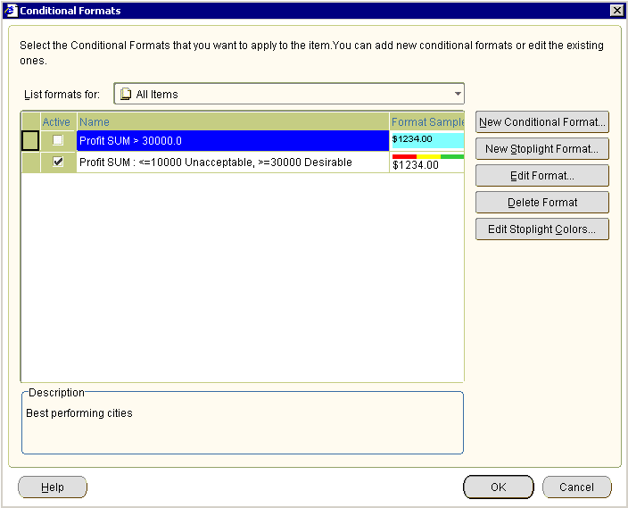
3. Choose Format | Conditional Formats to display the "Conditional Formats dialog".

   
   Description of the illustration d_cf3.gif
   
   

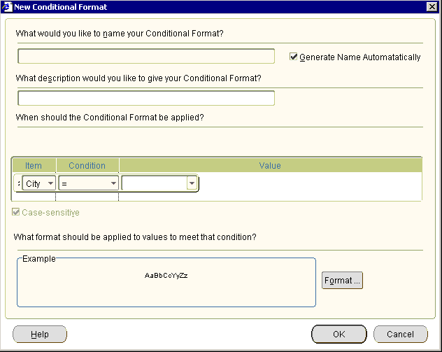
4. Click New Conditional Format to display the "New Conditional Format dialog".

   
   Description of the illustration d_cf4.gif
   
   

   Note: If you first selected a worksheet item in step 2, the worksheet item is selected by default in the Item field.

5. Specify how you want to highlight worksheet values, as follows:

   • (Optional) Use the What would you like to name your Conditional Format? field to create a user-friendly name for the format that will be used throughout Discoverer.

   • Use the When should the Conditional Format be applied? fields (i.e. Item, Condition, and Value) to create the condition that you want to apply.

     Hint: Use the Item field to select the worksheet item you want to format. Use the Format field to select the conditional operator (e.g. = for equals, > for greater than, < for less than) you want to use. Use the Value field to enter the value that you want to match against. For example, choose Profit SUM > 30,000 to highlight Profit SUM values that are greater than 30,000.

   • Click Format to display the "Format Data dialog: Format tab" dialog, which enables you to change the color of and text style for the worksheet value specified in the Item field.

6. Click OK to save changes that you have made and close the New Conditional Format dialog.

7. Click OK to close the Conditional Formats dialog.

   The worksheet is updated with the formatting changes that you have made.

Notes

• You can also create a conditional format in the following ways:

  • Select the Conditional Format option on the Formatting toolbar to display the "New Conditional Format dialog". For more information about toolbars, see "About the Formatting toolbar".

  • Right-click on the worksheet data area, and select the Conditional Format option to display the "Conditional Formats dialog", and click New Conditional Format.