Netra Data Plane Software Suite 1.1 User's Guide

This appendix provides guidelines for diagnosing and tuning network applications running under the Lightweight Runtime Environment (LWRTE) on UltraSPARC^® T1 processor multithreading systems.

Topics in this appendix include:

• Netra Data Plane Software Introduction
• UltraSPARC T1 Processor Overview
• Identifying Performance Issues
• Profiling Application Performance
• Profiling Metrics
• Optimization Techniques
• Tuning Troubleshooting
• Example Exercise

---

Netra Data Plane Software Introduction

The UltraSPARC T1 CMT systems deliver a strand-rich environment with performance and power efficiency that are unmatched by other processors. From a programming point of view, the UltraSPARC T1 processor's strand-rich environment can be thought of as symmetric multiprocessing on a chip.

The LWRTE provides an ANSI C development environment for creating and scheduling application threads to run on individual strands on the UltraSPARC T1 processor. With the combination of the UltraSPARC T1 processor and LWRTE, developers have an ideal platform to create applications for the fast path and the bearer-data plane space.

---

UltraSPARC T1 Processor Overview

The Sun UltraSPARC T1 processor employs chip multithreading, or CMT, which combines chip multiprocessing (CMP) and hardware multithreading (MT) to create a SPARC^® V9 processor with up to eight 4-way multithreaded cores for up to 32 simultaneous threads. To feed the thread-rich cores, a high-bandwidth, low-latency memory hierarchy with two levels of on-chip cache and on-chip memory controllers is available. FIGURE B-1 shows the UltraSPARC T1 architecture.

FIGURE B-1 UltraSPARC T1 Architecture

The processing engine is organized as eight multithreaded cores, with each core executing up to four strands concurrently. Each core has a single pipeline and can dispatch at most 1 instruction per cycle. The maximum instruction processing rate is 1 instruction per cycle per core or 8 instructions per cycle for the entire eight core chip. This document distinguishes between a hardware thread (strand), and a software thread (lightweight process (LWP)) in Solaris.

A strand is the hardware state (registers) for a software thread. This distinction is important because the strand scheduling is not under the control of software. For example, an OS can schedule software threads on to and off of a strand. But once a software thread is mapped to a strand, the hardware controls when the thread executes. Due to the fine-grained multithreading, on each cycle a different hardware strand is scheduled on the pipeline in cyclical order. Stalled strands are switched out and their slot in the pipeline given to the next strand automatically. Thus, the maximum throughput of 1 strand is 1 instruction per cycle if all other strands are stalled or parked. In general, the throughput is lower than the theoretical maximums.

The memory system consists of two levels of on-chip caching and on-chip memory controllers. Each core has level 1 instruction and data caches and TLBs. The instruction cache is 16 Kbyte, the data cache is 8 Kbyte, and the TLBs are 64 entries each. The level 2 cache is a 3 Mbyte unified instruction, and it is 12-way set associative and 4-way banked. The level 2 cache is shared across all eight cores. All cores are connected through a crossbar switch to the level 2 cache.

Four on-chip DDR2 memory controllers provide low-latency, high-memory bandwidth of up to 25 Gbyte per sec. Each core has a modular arithmetic unit for modular multiplication and exponentiation to accelerate SSL processing. A single floating-point unit (FPU) is shared by all cores, so this software is not optimal for floating-point intensive applications. TABLE B-1 summarizes the key performance limits and latencies.

---

Identifying Performance Issues

The key performance metric is the measure of throughput, usually expressed as either packets processed per second, or network bandwidth achieved in bits or bytes per second. In UltraSPARC T1 systems, the I/O limitation of 2 Gbyte per second puts an upper bound on the throughput metric. FIGURE B-2 shows the packet forwarding rate limited by this I/O bottleneck.

FIGURE B-2 Forwarding Packet Rate Limited by I/O Throughput

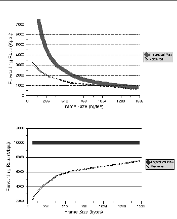
The theoretical max represents the throughput of 10 Gbyte per second. The measured results show that the achievable forwarding throughput is a function of packet size. For 64-byte packets, the measured throughput is 2.2 Gbyte per second or 3300 kilo packets per second.

In diagnosing performance issues, there are three main areas: I/O bottlenecks, instruction processing bandwidth, and memory bandwidth. In general, the UltraSPARC T1 systems have more than enough memory bandwidth to support the network traffic allowed by the JBus I/O limitation. There is nothing that can be done about the I/O bottleneck, so this document focuses on instruction processing limits.

For UltraSPARC T1 systems, the network interfaces are 1 Gbit and the interface is mapped to a single strand. In the simplest case, one strand is responsible for all packet processing from the corresponding interface. At a 1 Gbit line rate, 64-byte packets arrive at 1.44 Mpps (million packets per second) or one packet every 672 ns. To maintain this line rate, the processor must process the packet within 672 ns. On average, that is 202 instructions per packet. FIGURE B-3 shows the average maximum number of instructions the processor can execute per packet while maintaining line rate.

FIGURE B-3 Instructions per Packet Versus Frame Size

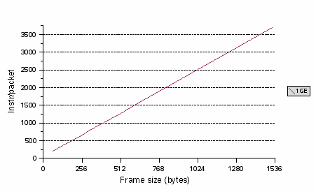
The inter-arrival time increases with packet size, so that more processing can be accomplished.

---

Profiling Application Performance

Profiling consists of instrumenting your application to extract performance information that can be used to analyze, diagnose, and tune your application. LWRTE provides an interface to assist you to obtain this information from your application. In general, profiling information consists of hardware performance counters and a few user-defined counters. This section defines the profiling information and how to obtain it.

Profiling is a disruptive activity that can have a significant performance effect. Take care to minimize profiling code and also to measure the effects of the profiling code. This can be done by measuring performance with and without the profiling code. One of the most disruptive parts of profiling is printing the profiling data to the console. To reduce the effects of prints, try to aggregate profiling statistics for many periods before printing, and print only in a designated strand.

The hardware counters are for the CPU, DRAM controllers, and JBus are described in TABLE B-2, TABLE B-3, and TABLE B-4 respectively.

instr_cnt

SB_full

FP_instr_cnt

IC_miss

DC_miss

ITLB_miss

DTLB_miss

L2_imiss

L2_dmiss_Id

mem_reads

mem_writes

bank_busy_stalls

rd_queue_latency

wr_queue_latency

rw_queue_latency

wr_buf_hits

jbus_cycles

dma_reads

dma_read_latency

dma_writes

dma_write8

ordering_waits

pio_reads

pio_read_latency

pio_writes

aok_dok_off_cycles

aok_off_cycles

dok_off_cycles

Each strand has its own set of CPU counters that only tracks its own events and can only be accessed by that strand. Only two CPU counters are 32 bits wide each. To prevent overflows, the measurement period should not exceed 6 seconds. In general, keep the measurement period between 1 and 5 seconds. When taking measurements, ensure that the application's behavior is in a steady state. To check this, measure the event a few times to see that it does not vary by more than a few percent between measurements. To measure all nine CPU counters, eight measurements are required. The application's behavior should be consistent over the entire collection period. To profile each strand on a 32-thread application, each thread must have code to read and set the counters. Sample code is provided in CODE EXAMPLE B-1. You must compile your own aggregate statistics across multiple strands or a core.

The JBus and DRAM controller counters are less useful. Since these resources are shared across all strands, only one thread should gather these counters.

The key user-defined statistic is the count of packets processed by the thread. Another statistic that can be important is a measure of idle time, which is the number of times the thread polled for a packet and did not find any packets to process.

The following example shows how to measure idle time. Assume that the workload looks like the following:

while(1)
   If( work_to_do ) {
	Do work
	Increment work_count
   } else {
	Increment idle_loop_count
   }
}

User-defined counters count the number of times through the loop no work was done. Measure the time of the idle loop by running idle loop alone (idle_loop_time). Then run real workload, counting the number of idle loops (idle_loop_count)

Idle_time = idle_loop_count * idle_loop_time

---

Profiling Metrics

You can calculate the following metrics after collecting the appropriate hardware counter data using the LWRTE profiling infrastructure. Use the metrics to quantify performance effects and help in optimizing the application performance.

• Instructions per cycle (IPC)

Calculate this metric by dividing instruction count by the total number of ticks during a time period when the thread is in a stable state. You can also calculate the IPC for a specific section of code. The highest number possible is 1 IPC, which is the maximum throughput of 1 core of the UltraSPARC T1 processor.

• Cycles per instructions (CPI)

This metric is the inverse of IPC. This metric is useful for estimating the effect of various stalls in the CPU.

• Instruction cache misses per instruction (IC_miss per instruction)

Multiplying this number with the L1 cache miss latency helps estimate the cost, in cycles, of instruction cache misses. Compare this to the overall CPI to see if this is the cause of a performance bottleneck.

• L2 instruction cache misses per instruction (L2_imiss per instruction)

This metric indicates the number of instructions that miss in the L2 cache, and enables you to calculate the contribution of instruction misses to overall CPI.

• Data cache misses per instruction (DC_miss per instruction)

Data cache miss rate in combination with the L2 cache miss rate quantifies the effect of memory accesses. Multiplying this metric with data cache miss latency provides an indication of its effect (contribution) on CPI.

• L2 cache misses per instruction (L2_miss per instruction)

Similar to data cache miss rate, this metric has higher cost in term of cycles of contribution to overall CPI. The metric also enables you to estimate the memory bandwidth requirements.

---

Optimization Techniques

Code Optimization

Writing efficient code and using the appropriate compiler option is the primary step in obtaining optimal performance for an application. Sun Studio 11 compilers provide many optimization flags to tune your application. Refer to the Sun Studio 11: C Users Guide for the complete list of optimization flags available. See Reference Documentation. The following list describes some of the important optimization flags that might help optimize an application developed with LWRTE.

• Inlining

Use the inline keyword declaration before a function to ensure that the compiler inlines that particular function. Inlining reduces the path length, and is especially useful for functions that are called repeatedly.

• Optimization level

The -xO[12345] option optimizes the object code differently based on the number (level). Generally, the higher the level of optimization, the better the runtime performance. However, higher optimization levels can result in longer compilation time and larger executable files. Use a level of -xO3 for most cases.

• -xtarget=UltraT1

This option indicates that the target hardware for the application is an UltraSPARC T1 CPU and enables the compiler to select the correct instruction latencies for that processor.

• -xprefetch and -xprefetch_level

Useful options if cache misses seem to be slowing down the application.

Pipelining

The thread-rich UltraSPARC T1 processor and the LWRTE programming environment enable you to easily pipeline the application to achieve greater throughput and higher hardware utilization. Pipelining involves splitting a function into multiple functions and assigning each to a separate strand, either on the same processor core or on a different core. You can program the split functions to communicate through Teja fast queues or channels.

One approach is to find the function with the most clock cycles per instruction (CPI) and then split that function into multiple functions. The goal is to reduce the overall CPI of the CPU execution pipeline. Splitting a large slow function into smaller pieces and assigning those pieces to different hardware strands is one way to improve the CPI of some subfunctions, effectively separating the slow and fast sections of the processing. When slow and fast functions are assigned to different strands, the CMT processor uses the execution pipelines more efficiently and improves the overall processing rate.

FIGURE B-4 shows how to split and map an application using fast queues and CMT processor to three strands.

FIGURE B-4 Example of Pipelining

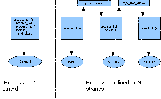
FIGURE B-5 shows how pipelining improves the throughput.

FIGURE B-5 Pipelining Effect on Throughput

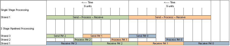
In this example, a single-strand application takes nine units of time to complete processing of a packet. The same application split into three functions and mapped to three different strands takes longer to complete the same processing, but is able to process more packets in the same time.

Parallelization

The other advantage of a thread-rich CMT processor is the ability to easily parallelize an application. If a particular software process is very compute-intensive compared to other processes in the application, you can allocate multiple strands to this processing. Each strand executes the same code but works on different data sets. For example, since encryption is a heavy operation, the application shown in FIGURE B-6 is allocated three strands for encryption.

FIGURE B-6 Parallelizing Encryption Using Multiple Strands

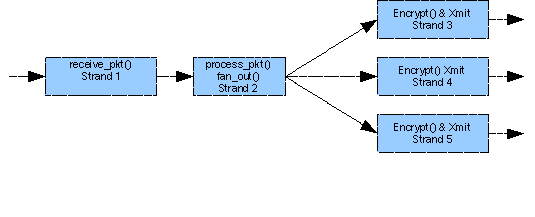
The process strand uses some well-defined logic to fan out encryption processing to the three encryption strands.

Packet processing applications that perform identical processing repeatedly on different packets easily lend themselves to this type of parallelization. Any networking protocol that is compute-bound can be allocated on multiple strands to improve throughput.

Mapping

Four strands share an execution pipeline in the UltraSPARC T1 processor. There are eight such execution pipes, one for each core. Determining how to map threads (LWRTE functions) to strands is crucial to achieving the best throughput. The primary goal of performance optimization is to keep the execution pipeline as busy as possible, which means trying to achieve an IPC of 1 for each processor core.

Profiling each thread helps quantify the relative processing speed of each thread and provide an indication of the reasons behind the differences. The general approach is to assign fast threads (high IPC) with slow threads on the same core. On the other hand, if instruction cache miss is a dominant factor for a particular function, then you would want to assign multiple instances of the same function on the same core. On UltraSPARC T1 processors you must assign any threads that have floating-point instructions to different strands if floating-point instructions are the performance bottleneck.

Parking Idle Strands

Often a workload does not have processing to run on every strand. For example, a workload has five 1 Gbit ports with each port requiring four threads for processing. This workload employs 20 strands for processing, leaving 12 strands unused or idle. You might run other applications on these idle strands but currently are testing only part of the application. LWRTE provides the options to park or to run while(1) loops on idle strands (that is, strands not participating in the processing).

Parking a strand means that there is nothing running on it and, therefore, the strand does not consume any of the processor's resources. Parking the idle strands produces the best result because the idle strands do not interfere with the working strands. The downside of parking strands is that there is currently no interface to activate a parked strand. In addition, activating a parked strand requires sending an interrupt to the parked strand, which might take hundreds of cycles before the strand is able to run the intended task.

If you want to run other processing on the idle strands, then parking these strands might result in optimistic performance measurements. When the final application is executed, the performance might be significantly lower than that measured with parked strands. In this case, running with a while(1) loop on the idle strands might be a more representative case.

The while(1) loop is an isolated branch. The while(1) loop executing on a strand takes execution resources that might be needed by the working strands on the same core to attain the required performance. while(1) loops only affect strands on the same core, they do not have an effect on strands on other cores. The while(1) loop often consumes more core pipeline resources than your application. Thus, if your working strands are compute-bound, running while(1) loops on all the idle strands is close to a worst case. In contrast, parking all the idle strands is the best case. To understand the range of expected performance, run your application with both parked and while(1) loops on the idle strands.

Slow Down Polling

As explained in Parking Idle Strands, strands executing on the same core can have both beneficial and detrimental effects on performance due to common resources. The while(1) loop is a large consumer of resources, often consuming more resources than a strand doing useful work. Polling is very common in LWRTE threads and, as seen with the while(1) loop, might waste valuable resources needed by the other strands on the core to achieve performance. One way to alleviate the waste by polling is to slow down the polling loop by executing a long latency instruction. This situation causes the strand to stall, making its resources available for use by the other strands on the core. LWRTE exports interfaces to slowing down the polling that include:

• Access the memory location using a little endian load (ASI_PRIMARY_LITTLE). This option always goes to L2 and takes about 30 cycles.
• Meaningless CAS, which takes about 39 cycles.
• Meaningless PIO.
• ASI register read.
• Floating-point instructions.

The method you select depends on your application. For instance, if your application is using the floating-point unit, you might not want a useless floating-point instruction to slow down polling because that might stall useful floating-point instructions. Likewise, if your application is memory bound, using a memory instruction to slow polling might add memory latency to other memory instructions.

---

Tuning Troubleshooting

What Is a Compute-Bound Versus a Memory-Bound Thread?

A thread is compute-bound if its performance is dependent on the rate the processor can execute instructions. A memory-bound thread is dependent on the caching and memory latency. As a rough guideline for the UltraSPARC T1 processor, the CPI for a compute-bound thread is less than five and for a memory-bound thread is considerably higher than five.

Can't Reach Line Rate for Packets Smaller Than 300 Bytes

Single-thread receives, processes, and transmits packets can only achieve line rate for 300 byte packets or larger.

Goal: Want to get line rate for 250 byte packets.

Solution: Need to optimize single-thread performance. Try compiler optimization, different flags -O2, -O3, -O4, -O5, fast function inlining. Change code to optimize hot sections of code, you might need to do profiling.

Goal: Want to get to line rate for 64-byte packets.

Solution: Parallelize or pipeline. To get from 300 to 64-byte packets running at line rate is probably too much for just optimizing single-thread performance.

Can't Scale Throughput to Multiple Ports

When you increase the number of ports the results don't scale. For example, with a line rate of 400 byte packets with two interfaces, when you increase to three interfaces, you get only 90% of line rate.

Solution: If the problem is in parallelizing, determine if there are conflicts for shared resources, or synchronization and communication issues. Are there any lock contention or shared data structures? Is there a significant increase in CPI, cache misses, or store buffer full cycles? Are you using the shared resources such as the modular arithmetic unit or floating-point unit? Is the application at the I/O throughput bottleneck? Is the application at the processing bottleneck?

If there is a conflict for pipeline resources, optimizing single-thread performance would use fewer resources and improve overall throughput and scaling. In this situation, distribute the threads across the cores in a more optimal fashion or park unused strands.

How Do I Achieve Line Rate for 64-byte Packets?

The goal is to achieve line rate processing on 64-byte packets for a single 1 Gigabit Ethernet port. The current application requires 575 instructions per packet executing on 1 strand.

Solution: A 64-byte packet size has 202 instructions per packet. So optimizing your code will not be sufficient. You must parallelize or pipeline. In parallelization, the task is executed in multiple threads, each thread doing the identical task. In pipelining, the task is split up into smaller subtasks, each running on a different thread, that are sequentially executed. You can use a combination of parallelization and pipelining.

In parallelization, parallelize the task N ways, to increase the instructions per packet N times. For example, execute the task on three threads, and each thread can now have 606 instructions per packet (202 x 3) and still maintain 1 Gbit line rate for 64-byte packets. If the task requires 575 instructions per packet, run the code on 3 threads (606 instruction per packet), to achieve 1 Gbit line rate for 64-byte packets. Parallelizing maximizes the throughput by duplicating the application on multiple strands. However, some applications cannot be parallelized or depend too much upon synchronization when executed in parallel. For example, the UltraSPARC T1 network driver is difficult to parallelize.

In pipelining, you can increase the amount of processing done on each packet by partitioning the task into smaller subtasks that are then run sequentially on different strands. Unlike parallelization, there are not more instructions per packet on a given strand. Using the example from the previous paragraph, split the task into three subtasks, each executing up to 202 instructions of the task. In both the parallel and pipelined cases, the overall throughput is similar at three packets every 575 instructions. Similar to parallelization, not all applications can easily be pipelined and there is overhead in passing information between the pipe stages. For optimal throughput, the subtasks need to execute in approximately the same time, which is often difficult to do.

When Should I Consider Thread Placement?

Thread placement refers to the mapping of threads onto strands. Thread placement can improve performance if the workload is instruction-processing bound. Thread placement is useful in cases where there are significant sharing or conflicts in the L1 caches, or when the compute-bound threads are grouped on a core. In the case of conflicts in the L1 caches, put the threads that conflict on different cores. In the case of sharing in the L1 caches, put the threads that share on the same core. In the case of compute-bound threads fighting for resources, put these threads on different cores. Another method would be to place high CPI threads together with low CPI threads on the same core.

Other shared resources that might benefit from thread placement include TLBs and modular arithmetic units. There are separate instruction and data TLBs per core. TLBs are similar to the L1 caches in that there can be both sharing and conflicts. There is only one modular arithmetic unit per core, so placing threads using this unit on different cores might be beneficial.

---

Example Exercise

This section uses the reference application RLP to analyze the performance of two versions of an application. The versions of the application are functionally equivalent but are implemented differently. The profiling information helps to make decisions regarding pipelining and parallelizing portions of the code. The information also enables efficient allocation of different software threads to strands and cores.

Application Configuration

The RLP reference application has three basic components:

• PDSN
• ATIF
• RLP

The PDSN and ATIF each have receive (RX) and transmit (TX) components. A Netra T2000 system with four in-ports and four out-ports was configured the four instances of the RLP application. FIGURE B-7 describes the architecture.

FIGURE B-7 RLP Application Setup

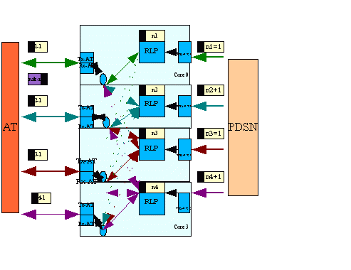
In the application, the flow of packets from PDSN to AT is the forward path. The RLP component performs the main processing. The PDSN receives packets (PDSN_RX) and forwards the packets to the RLP strand. After processing the packet header, the RLP strand forwards the packet to the AT strand for transmission (ATIF_TX). Summarizing:

• -> PDSN_RX -> RLP -> ATIF_TX -> (forward path)
• <- PDSN_TX <- RLP <- ATIF_RX <- (reverse path)

The example focuses on the forward path performance only.

Configuration 1

In configuration 1, the PDSN, ATIF, and RLP functionality is assigned to different threads as shown in TABLE B-5.

Configuration 2

In configuration 2, the PDSN and ATIF functionality is split into separate RX and TX functions and assigned to different strands as shown in TABLE B-6.

PSDN_RX_0

PSDN_RX_1

PSDN_RX_2

PSDN_RX_3

while(1)

while(1)

PSDN_TX_1

while(1)

RLP_0

RLP_1

RLP_2

RLP_3

while(1)

while(1)

PSDN_TX_2

while(1)

ATIF_RX_0

ATIF_RX_1

ATIF_RX_2

ATIF_RX_3

while(1)

while(1)

PSDN_TX_3

ATIF_TX_0

ATIF_TX_1

ATIF_TX_2

ATIF_TX_3

while(1)

PSDN_TX_0

while(1)

Using the Profiling API

It is important to understand hardware counter data collected from the strands that have been assigned some functionality. The strands assigned while(1) loops take up CPU resources but are not analyzed in this study. This study analyzes overall thread performance by sampling hardware counter data. After the application has reached a steady state, the hardware counters are sampled at predetermined intervals. Sampling reduces the performance perturbations of profiling and averages out small differences in the hardware counter data collected. In both versions of the application, the profiling affected performance by about 5-7% in overall throughput. The goal is to have the application in a steady state with profiling on.

The analysis uses the Teja Profiling API (refer to the Netra Data Plane Software Suite 1.1 Reference Manual) and creates a simple function that collects hardware counter data for all the available counters per strand. The function is called from a relevant section of the application. The hardware counter data is related to application performance as the number of packets processed by the application-defined counter that is passed to the Teja API. To reduce the performance impact of profiling, the profiling API is not called for each packet processed. For the RLP application and Netra T2000 hardware combination, the API is called every five seconds, otherwise the counters overflow.

The pseudo-code in CODE EXAMPLE B-1 shows the functions that were created to collect the hardware counter data.

#ifdef TEJA_PROFILE
/* some global vars */
int event[MAX_CPUS];
uint64_t start_profile_value[MAX_CPUS]; /* when  to start collection hw counter data */
uint64_t update_interval_value[MAX_CPUS]; /* when to move to the next counter */
int number_profile_samples[MAX_CPUS]; /* number of samples to be taken before dumping */
int dump_enable[MAX_CPUS]; /* 0 = Dump Disabled 1 = Dump enabled */
int samples_collected[MAX_CPUS]; /* running count of samples collected */
/* set up control values for collection all CPU hardware counter */
inline void init_profiler(uint64_t start_val, uint64_t interval, int num_samples){
  int cpuid = teja_get_cpu_number();
  event[cpuid] = 1;
  number_profile_samples[cpuid] = num_samples;
  start_profile_value[cpuid] = start_val;
  update_interval_value[cpuid] = interval;
  dump_enable[cpuid] = 0;
  samples_collected[cpuid] = 0;
}
/* pass the value to be compared against for control */
/* this can be time/packet count */
inline void collect_profile(uint64_t user_value){
  int ret;
  int cpuid = teja_get_cpu_number();
  if (user_value ==  start_profile_value[cpuid] ) {
    ret = teja_profiler_start(TEJA_PROFILER_CMT_CPU, event[cpuid] );
    if (ret == -1)
      printf("Error Starting Profile \n");
  }
  if ((user_value % update_interval_value[cpuid] )==0) {
    ret = teja_profiler_update(TEJA_PROFILER_CMT_CPU, user_value);
    if (ret == -1)
      printf("Error Updating Profile \n");
    event[cpuid] = event[cpuid] * 2 ;
    if (event[cpuid]==256){
      event[cpuid] = 1; 
      samples_collected[cpuid]++;
      if (samples_collected[cpuid] == number_profile_samples[cpuid] ){
	dump_enable[cpuid] = 1;
	/* there is a race here but the side effect is benign as Teja should print*/
	/* appropriate records when things get over-written */
	samples_collected[cpuid] = 0;
      }
    }
    /* 256 is 2^8 8 is number of HW counter in N1 */
    ret = teja_profiler_start(TEJA_PROFILER_CMT_CPU, event[cpuid] );
    if (ret == -1) 
      printf ("Error Starting  Profiler\n");
  }
}
inline void
dump_hw_profile(){
  int cpuid;
  for (cpuid = 0 ; cpuid < MAX_CPUS ; cpuid++){
    if (dump_enable[cpuid] == 1){ 
      teja_profiler_dump(cpuid);
      dump_enable[cpuid] = 0; 
    } 
  }
}
#endif

The code uses the teja_profiling_api to create a simple set of functions for collecting hardware counter data. The code is just one example of API usage, but it is a very good starting point for performance analysis of a LWRTE application.

Each strand that does useful work is annotated with a call to the collect_profile() function and is passed the number of packets that have been processed. The location in the code where the call is made is important. In this application, the call is made in the active section of the code where a packet returned is not null. The init_profiler() function call sets up the starting point, an interval, and number of samples to be collected. The dump_hw_profile() function is called in the statistics strand and prints the data to the console.

Profiling Data

The API calls teja_profile_start and teja_profiler_update to set up and collect a specific pair of hardware counters. The call to teja_profile_dump outputs the collected statistics to the console. These function calls are in bold in CODE EXAMPLE B-1. For a detailed description of these API functions refer to the Netra Data Plane Software Suite 1.1 Reference Manual.

A sample output based on the code in CODE EXAMPLE B-1 is shown in CODE EXAMPLE B-2.

PROFILE_DUMP_START,ver,1.1
CPUID,ID,Type,Cycles,PC,Grp,Evt_Hi,Evt_Lo,Overflow,User Data
4,6043,2,30051d74250,512598,1,3a372e12,dc22fb0,0,30c1b080
4,1fad3,1,30051d74c70,525968,1,100,2
4,6043,2,3021dd890b0,512598,1,3a3215c1,0,0,30e03500
4,1fad3,1,3021dd89abc,525968,1,100,4
4,6043,2,303e9d9e3e0,512598,1,3a2ee368,15561,0,30feb980
4,1fad3,1,303e9d9ee4c,525968,1,100,8
4,6043,2,305b5db43b0,512598,1,3a2ef375,29d8db7,0,311d3e00
4,1fad3,1,305b5db4db0,525968,1,100,10
4,6043,2,30781dc9ae0,512598,1,3a2f5793,0,0,313bc280
4,1fad3,1,30781dca544,525968,1,100,20
4,6043,2,3094dddeb10,512598,1,3a303d12,0,0,315a4700
4,1fad3,1,3094dddf51c,525968,1,100,40
4,6043,2,30b19df3258,512598,1,3a2ebfbf,6774,0,3178cb80
4,1fad3,1,30b19df3ccc,525968,1,100,80
4,6043,2,30ce5e08248,512598,1,3a2eb2aa,8c9c8f,0,31975000
4,1fad3,1,30ce5e08e24,525968,1,100,1
4,6043,2,30eb1e1e37c,512598,1,3a2f090e,dbbe5ae,0,31b5d480
4,1fad3,1,30eb1e1eea0,525968,1,100,2
4,6043,2,3107de334a8,512598,1,3a2f958f,0,0,31d45900
4,1fad3,1,3107de33f9c,525968,1,100,4
4,6043,2,31249e48ba8,512598,1,3a2fe948,1564a,0,31f2dd80
PROFILE_DUMP_END

All the numbers in the output are hexadecimal. This format can be imported into a spreadsheet or parsed with a script to calculate the metrics discussed in Profiling Metrics. The output in CODE EXAMPLE B-2 shows two types of records that correspond to teja_profile_start and teja_profile_update calls.

• An example of a teja_profile_start record:


4,1fad3,1,30051d74c70,525968,1,100,2

This record is formatted as: CPUID, ID, Call Type, Tick Counter, Program Counter, Group Type, Hardware counter 1 code, and Hardware counter 2 code. There is one such record for every call to teja_profiler_start indicated by a 1 in the Call Type (third) field.

• An example of a teja_profile_update record:


4,6043,2,31249e48ba8,512598,1,3a2fe948,1564a,0,31f2dd80

This record is formatted as: CPUID, ID, Call Type, Tick Counter, Program Counter, Group Type, Counter Value 1, Counter Value 2, Overflow Indicator and user defined data. There is one such record for every call to teja_profile_update indicated by a 2 in the Call Type field.

Metrics

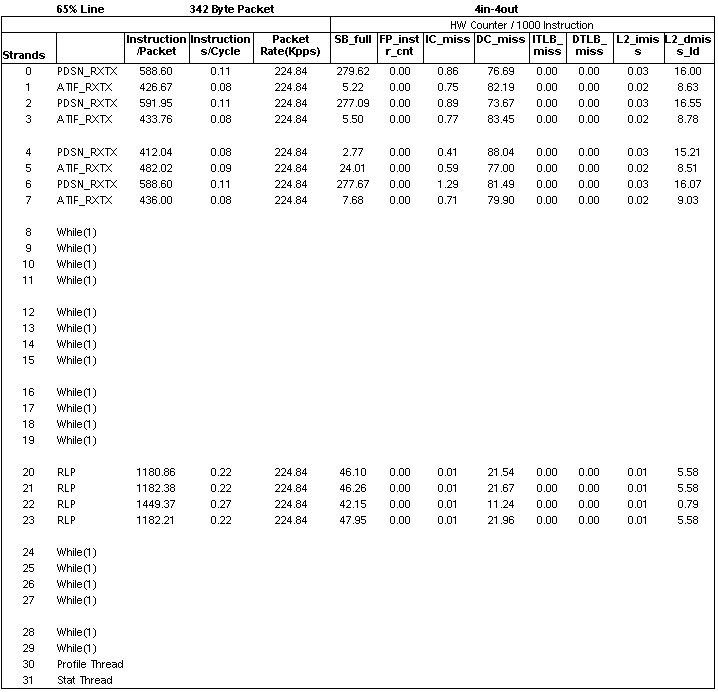
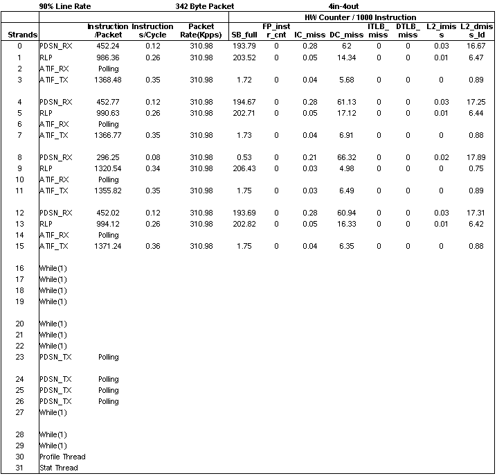
The data from the output is processed using a spreadsheet to calculate the metrics per strand as presented in TABLE B-7.

These metrics in TABLE B-7 provide insight into the performance of each strand and of each core.

Results

Configuration 1

Configuration 1 sustained 224 kpps (kilo packets per second) on each of the four flows or 65% of 1 Gbps line rate for a 342 byte packet. Only three cores of the UltraSPARC T1 processor were used to achieve this throughput. See FIGURE B-8.

FIGURE B-8 Results From Configuration 1

Configuration 2

Configuration 2 sustained 310 kpps (kilo packets per second) on each of the four flows or 90% of 1 Gbps line rate for a 342 byte packet. Four cores of the UltraSPARC T1 processor were used to achieve this throughput. The Polling notation implies that the ATIF_RX thread was allocated to a strand, but no packets were handled by that thread during the test. See FIGURE B-9.

FIGURE B-9 Results From Configuration 2

Analysis

When comparing the processed hardware counter information it is necessary to co-relate that data with the collection method. The counter information was sampled over the steady-state run of the application. There are other methods to collect hardware counter data that enable you to optimize a particular section of the application.

Comparing the Instruction per Cycle columns from the two tables shows that RXTX threads in configuration 1 are slower than the split RX and TX threads in configuration 2. The focus is on the forward path processing. Consider the following:

• For configuration 1 - PDSN_RXTX -> RLP -> ATIF_RXTX
• For configuration 2 - PDSN_RX -> RLP -> ATIF_TX

The main bottleneck in configuration 1 is the combined ATIF_RXTX thread that runs at the slowest rate, taking about 12 cycles per instruction. In configuration 2, ATIF_RX is moved to another strand and the bottleneck in the forward path (that does not need ATIF_RX) is removed, allowing ATIF_TX to run at a considerably faster 2.82 cycles per instruction. Also in configuration 2, using another strand speeded up the slowest section of pipelined processing. To speed up this configuration even more would require optimizing PDSN_RX, which is now the slowest part of the pipeline taking up 8.53 cycles per instruction. This optimization can be accomplished by optimizing code to reduce the number of instructions per packet or by splitting up this thread using more strands.

To explain the high CPI of the ATIF_RXTX strand in configuration 1, note that there are 82 DC_misses (dcache misses) per 1000 instructions as compared to just six misses in the ATIF_TX of configuration 2. You can estimate the effect of these misses by calculating the number of cycles these misses add to overall processing. Use information from TABLE B-1 to calculate the worst case effect of the data cache and L2 cache misses. The results for these calculations are shown in TABLE B-8 for configuration 1 and in TABLE B-9 for configuration 2.

The highlighted rows show that the CPI contribution of dcache and L2 cache misses in configuration 1 is much higher than configuration 2, making the ATIF_RXTX strand much slower.

There are other effects involved here besides those outlined in the preceding tables. The move to put the RLP on the same core as PDSN_RX and ATIF_TX causes constructive sharing in the level 1 instruction and data caches as seen in the DC_misses per 1000 instructions for RLP strand. Another effect is that the slower processing rate of configuration 1 causes the RLP strand to spin on null more often, increasing the number of instruction per packet metric and slowing down processing. Other experiments have shown that threads that poll or do the while(1) loop take away processing bandwidth from other more useful threads.

In conclusion, configuration 2 achieves a higher throughput because the ATIF processing was split to RX and TX and each was mapped to a different strand, effectively parallelizing the ATIF thread. Configuration 2 used more strands, but was able to achieve much higher throughput.

Other Uses

The same teja_profiling_api can be used in another way to evaluate and understand the performance of an application. Besides the sampling method outlined in the preceding section, you can use the API to profile specific sections of the code. This type of profiling enables you to make decisions regarding pipelining and reorganizing memory structures in the application.

^{1 (TableFootnote) Tcc instructions that are cancelled due to encountering a higher-priority trap are still counted.}

^{2 (TableFootnote) SB_full increments every cycle a strand (virtual processor) is stalled due to a full store buffer, regardless of whether other strands are able to keep the processor busy. The overflow trap for SB_full is not precise to the instruction following the event that occurs when ovfl is set. The trap might occur on the instruction following the event or the following two instructions.}

^{3 (TableFootnote) Only floating-point instructions that execute in the shared FPU are counted. The following instructions are executed in the shared FPU: FADDS, FADDD, FSUBS, FSUBD, FMULS, FMULD, FDIVS, FDIVD, FSMULD, FSTOX, FDTOX, FXTOS, FXTOD, FITOS, FDTOS, FITOD, FSTOD, FSTOI, FDTOI, FCMPS, FCMPD, FCMPES, FCMPED.}

^{4 (TableFootnote) L2 misses because stores cannot be counted by the performance instrumentation logic.}

Netra Data Plane Software Suite 1.1 User's Guide

820-2374-10

Copyright © 2007, Sun Microsystems, Inc. All Rights Reserved.