Understanding Yield Curves
Yield Curves incorporate data from various market sources, such as Bloomberg, Reuters, and Telerate, by using the Extract-Transform-Load (ETL) process. You can use the ETL process to use user-defined source data for developing yield curves. You can specify the origin of the source data, define generic bond market volatility, credit spread, currency source data, and identify the type of data that you use to create the curves. Once you specify the source data for your curves, you then specify the curve interpolation methods to define how to interpret the source data.
There are two engines used to define yield curves, the Curve Generator application engine and the Curve Evaluator application engine.
The Curve Generator component enables you to set up the rules for interpolating a set of data points. Once you establish the setup rules, you can add, modify, or delete these rules. You do not need to set up new rules each time the Curve Generator component processes information.
The Curve Evaluator component is a process called by other support modules. This component is an online module that calculates rates as requested by other FSI applications. When the Curve Evaluator application engine receives a set of parameters from the calling application, the Curve Evaluator application engine calculates the requested rates and returns them to the calling application.
Common Concepts
The pages used to set up Yield Curves all share common concepts. This section discusses those concepts:
Curve interpolation.
Bootstrapping.
Short-term yields.
Issue types and frequencies.
Derived data.
Curve Interpolation
The Curve Generator application engine supports the following interpolation methods:
Hermite cubic: Creates a sequence of cubic equations between each data point.
These cubic equations are controlled by the change in the curve at the two end points.
Cubic spline: Creates a set of cubic equations like the hermite cubic, but the cubic spline guarantees that both the change in the curve and the rate of change at the quoted points (the slope and curvature of the function) remain constant.
If you select this interpolation type, you need to further specify the way that the spline curve handles the left and right end points of each data set. This is done by modifications to individual equations that comprise the contiguous segments of the yield curve. Options are:
Continuous curl: The change in curvature, or curl, is made continuous between the first and second, and penultimate and last points of the data set.
Curvature constraint: Describes the behavior of the graphed point over the domain, enabling you to specify the degree of curvature at the first and last points of the data set.
Slope constraint: Enables you to specify the slope at the endmost points.
Linear segments: Creates straight lines between each succeeding pair of quoted yields.
Step function: Creates a yield curve from a given data point that looks like horizontal line segments.
Until specifying a new yield, the step function uses the exact same yield for all subsequent maturities. This function can be very useful when referencing the prime rate because it has no maturity component. The Step function ignores the current term structure, therefore, no meaningful term information can be derived from it.
Interpolations are used on the Derived Data page and more specifically on the curve interpolation pages.
Bootstrapping
Using a technique called bootstrapping, the Curve Generator can take a coupon that is bearing market issue, strip its future cash flows (coupon payments) and convert them into a set of zero-coupon bearing market issues. To initiate bootstrapping, assign a coupon frequency to the coupon that is bearing market issue. If you do not select a coupon frequency value in the Market Issues page, the Curve Generator assumes that the market issue is non-coupon bearing. Once you set up the appropriate data in the Market Issues page, the Curve Generator can interpret the differences between zero-coupon market yields and coupon-paying yields.
Short-Term Yields
You must specify an overnight or short-term yield if you need rates from a given yield curve within maturities that are shorter than those that are in the source data. For example, source information from the data set includes a 30-day maturity point that is given by a treasury bill. However, when you require a term structure that includes maturities for overnight, two days, three days, one week, and so on, you must define those points with data that you determine is appropriate for those points. The Overnight Fed Funds is a commercial rate that is available if you do not have an inhouse funding curve with a more desirable set of data points for defining those short-term maturities.
Issue Types and Frequencies
You define issue types and frequencies on the Market Issues page. The issue types and frequencies available for use are as follows:
Singular issues: When the issue type is singular, the pricing information for the exact instrument that the CUSIP code designates becomes active and is later used for data set information.
Singular issues do not have a predefined issue calendar and typically are nonstandard financial instruments. For example, bank notes are short-term money-market debt instruments that are issued in various denominations and maturities. Each bank note has a unique value, and the institution attaches a CUSIP code to track it.
Repeating issues: The most recent issuance (also called on the run issuance) for a market issue is used to designate the data set point.
Repeating issues have an anticipated frequency. For example, treasury notes have standard value and maturity, and they use the most recently issued instruments when building a yield curve. If you specify the market issue as a repeating issue, you must also set up an issue frequency and nominal tenor.
Issue frequency: Indicates the periodicity for the issuance (for example, 52-week treasury bills are issued every 30 days).
Nominal tenor: A surrogate tenor.
Periodically organizations offer new security issues for notes and bonds. The nominal tenor acts as a surrogate tenor for these products according to their properties. A treasury bill, for example, may have an actual maturity of 28 days from issuance, but the nominal tenor assigned to this product may be 30 days. This facilitates the construction of term structures such as the Treasury Curve.
Derived Data
Derived data creates composite curves from multiple sources. Use the Derived Data page to define curves that are derived from operations performed on multiple curves. For example, you might define a term structure of credit spreads as the difference between a term structure of corporate bonds and the risk-free curve.
Alternatively, you can create curves by performing operations on two or more existing curves and designating the interpolation method that provides the desired result. For example, you can create a term structure by averaging the LIBOR and CD yields to comprise the overnight to two-year rates and arrive at the two-to-ten-year rate by using treasury notes and positively shifting by 150 basis points. By including the 30-year treasury bond rate, you can complete construction of the newly defined curve. A credit spread curve can be constructed by subtracting the risk-free curve from a curve that is composed of corporate bonds.
Note: The risk free curve is typically defined by the Treasury Curve. You can define the risk-free curve according to your business practices.
The lag frequency defines a historic period of time when you want your calculation to begin.
The lag frequency period is not included in the rolling average interest rate calculation unless the value is set to zero. For example, if today is February 2002, and you set the lag frequency to three months and the rolling average frequency to eight months, the application calculates the rolling average from November 2001 to April 2001. The lag period from February 2002 to December 2002 is not included in the interest rate calculation.
A rolling average, also called a moving average, is an average of a series of numbers that is recomputed regularly by adding the most recent data and dropping the oldest one. Some Funds Transfer Pricing methodologies recommend using a rolling average to calculate the transfer price for indeterminate deposits. This provides a smoother, more consistent rate and argues that it's more representative of the cost of funding rather than using a more volatile daily rate.
A rolling average frequency defines the span of time that is being used to calculate a rolling average.
The data within this time span is used to calculate the rolling average rates. Rolling averages are based on existing rolling average rates. A rolling average can only be calculated based on a previously defined data set.
Note: Because the Treasury Curve comprises issues varying in maturity from an overnight to a 30-year bond, nominal tenors are specified for each treasury product that you want to use in constructing curves. This eliminates the need for an exact day count for each issue every time that you want to construct a yield curve.
Understanding Rolling Average Calculations within the Yield Curve Generator
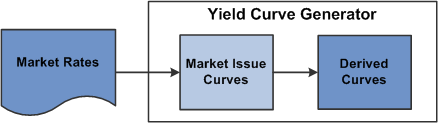
In order to create derived yield curves, market rates are first loaded to the rate tables (PS_YC_RATE_HDR and PS_YC_RATE_TBL), either using the ETL process or data entry pages. Running the Yield Curve Generator creates the market issue curves then the derived curves based off of those market issue curves. The output of both curve types is stored in the PS_YC_PNEQS table.
Image: Derived Yield Curve Overview
This example illustrates the fields and controls on the Derived Yield Curve Overview. You can find definitions for the fields and controls later on this page.
As stated earlier, a rolling average is an average of a series of rates that is recomputed regularly by adding the most recent data and dropping the oldest one. PeopleSoft Interest Rate Environment uses a simple rolling average method, which is the unweighted mean of the previous 'n' data points. For example, the formula for a five day rolling average appears as follows:
Image: Formula for Five Day Rolling Average
This example illustrates the fields and controls on the Formula for Five Day Rolling Average. You can find definitions for the fields and controls later on this page.
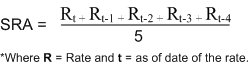
Note that the denominator is dependant upon the number of data points you have loaded into the system rather than the number of days in your rolling average frequency. This is important for rolling averages calculated on more than five days since market rates are not available for weekends and holidays. Thus, if you have a 30 day rolling average the time span that the Yield Curve Generator searches is between t and t-29, but will calculate the average based on the number of rates it finds (which in a normal month is approximately 22 when you exclude eight weekend days).
Known Data Points (Market Issue Points)
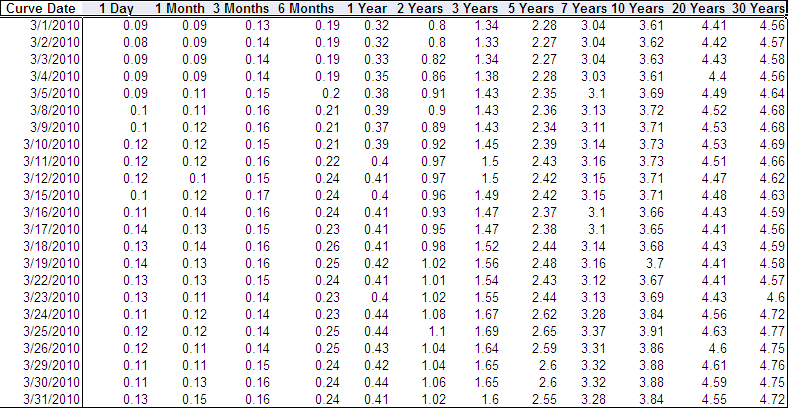
The following table displays the base market rates that were sourced from the Treasury and processed in the Market Issue Curve (TREAS_SET1) table; these are the rates that the Yield Curve Generator uses to calculate the rolling average.
Image: Base Market Rates
This example illustrates the fields and controls on the Base Market Rates.
The next figure displays the 30 day rolling average calculations for all known points (which are the rates at each of the market issues) and for the 3/31/10 curve:
Image: Rolling Average Calculation
This example illustrates the fields and controls on the Rolling Average Calculation.
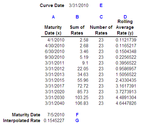
Column A represents the Maturity Date for each Market Issue.
Column B represents the sum of the rates for each Market Issue from 3/1/10 – 3/31/10.
Column C represents the number of data points sourced from the Treasury and loaded into the system.
Column D represents the average of the series 3/1/10 – 3/31/10 for each Market Issue, or Column B / Column C.
For each maturity date in Column A, the rolling average rate in Column D will tie to the yield rates on the View Yield Curve page.
Interpolated Points
Linear interpolation is a method of curve fitting using linear polynomials. If two known points are provided by the coordinates (x0, y0) and (x1, y1), the linear interpolant is the straight line between these points.
Image: Linear Interpolation - Coordinates
This example illustrates the fields and controls on the Linear Interpolation - Coordinates. You can find definitions for the fields and controls later on this page.
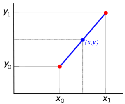
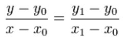
In the graph above, the blue line represents the linear interpolant as determined by the two red points, and the value y at x may be found by linear interpolation. The algebraic expression is as follows:
Image: Algebraic Expression of Linear Interpolation Method
This example illustrates the fields and controls on the Algebraic Expression of Linear Interpolation Method. You can find definitions for the fields and controls later on this page.
If you solve for y, which is the unknown value at x, the expression appears as follows:
Image: Algebraic Expression of Linear Interpolation Method as solved for Y
This example illustrates the fields and controls on the Algebraic Expression of Linear Interpolation Method as solved for Y. You can find definitions for the fields and controls later on this page.
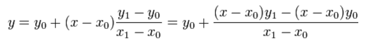
You can use the above formulas to check the interpolated rate or you can use MicroSoft Excel, which makes use of the same mathematics in its Forecast function:
=FORECAST(Maturity Date (F) ,
OFFSET(Rates (D),MATCH(Maturity Date (F) ,Maturity Date (A),1)-1,0,2),
OFFSET(Maturity Date (A) ,MATCH(Maturity Date (F) ,Maturity Date (A),1)-1,0,2))
Setting Up Rolling Averages
To set up rolling averages:
Define derived data parameters on the Data Source page.
Define yield curve, interpolant, rolling average, and rolling average frequency parameters on the Derived Data page.
Note: You can also define lag frequency on the Derived Data page, but it is optional.
See Derived Data Page.
Associate the data set to the yield curve on the Curve Interpolants page.