4.2.9 Building a k-Means Model
The ore.odmKM function uses the Oracle Data Mining k-Means (KM) algorithm, a distance-based clustering algorithm that partitions data into a specified number of clusters. The algorithm has the following features:
-
Several distance functions: Euclidean, Cosine, and Fast Cosine distance functions. The default is Euclidean.
-
For each cluster, the algorithm returns the centroid, a histogram for each attribute, and a rule describing the hyperbox that encloses the majority of the data assigned to the cluster. The centroid reports the mode for categorical attributes and the mean and variance for numeric attributes.
For information on the ore.odmKM function arguments, invoke help(ore.odmKM).
Example 4-19 Using the ore.odmKM Function
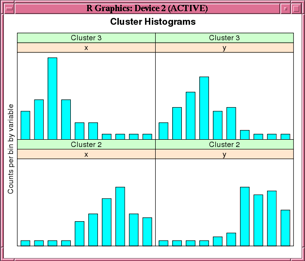
This example demonstrates the use of the ore.odmKMeans function. The example creates two matrices that have 100 rows and two columns. The values in the rows are random variates. It binds the matrices into the matrix x, then coerces x to a data.frame and pushes it to the database as x_of, an ore.frame object. The example next invokes the ore.odmKMeans function to build the KM model, km.mod1. It then invokes the summary and histogram functions on the model. Figure 4-3 shows the graphic displayed by the histogram function.
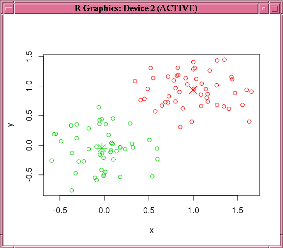
Finally, the example makes a prediction using the model, pulls the result to local memory, and plots the results.Figure 4-4 shows the graphic displayed by the points function.
x <- rbind(matrix(rnorm(100, sd = 0.3), ncol = 2),
           matrix(rnorm(100, mean = 1, sd = 0.3), ncol = 2))
colnames(x) <- c("x", "y")
x_of <- ore.push (data.frame(x))
km.mod1 <- NULL
km.mod1 <- ore.odmKMeans(~., x_of, num.centers=2)
summary(km.mod1)
histogram(km.mod1)
# Make a prediction.
km.res1 <- predict(km.mod1, x_of, type="class", supplemental.cols=c("x","y"))
head(km.res1, 3)
# Pull the results to the local memory and plot them.
km.res1.local <- ore.pull(km.res1)
plot(data.frame(x=km.res1.local$x, y=km.res1.local$y),
                col=km.res1.local$CLUSTER_ID)
points(km.mod1$centers2, col = rownames(km.mod1$centers2), pch = 8, cex=2)
head(predict(km.mod1, x_of, type=c("class","raw"),
             supplemental.cols=c("x","y")), 3)
Listing for Example 4-19
R> x <- rbind(matrix(rnorm(100, sd = 0.3), ncol = 2),
+             matrix(rnorm(100, mean = 1, sd = 0.3), ncol = 2))
R> colnames(x) <- c("x", "y")
R> x_of <- ore.push (data.frame(x))
R> km.mod1 <- NULL
R> km.mod1 <- ore.odmKMeans(~., x_of, num.centers=2)
R> summary(km.mod1)

Call:
ore.odmKMeans(formula = ~., data = x_of, num.centers = 2)

Settings:
                         value
clus.num.clusters            2
block.growth                 2
conv.tolerance            0.01
distance             euclidean
iterations                   3
min.pct.attr.support       0.1
num.bins                    10
split.criterion       variance
prep.auto                   on

Centers:
            x           y
2  0.99772307  0.93368684
3 -0.02721078 -0.05099784
R> histogram(km.mod1)
R> # Make a prediction.
R> km.res1 <- predict(km.mod1, x_of, type="class", supplemental.cols=c("x","y"))
R> head(km.res1, 3)
            x          y CLUSTER_ID
1 -0.03038444  0.4395409          3
2  0.17724606 -0.5342975          3
3 -0.17565761  0.2832132          3
# Pull the results to the local memory and plot them.
R> km.res1.local <- ore.pull(km.res1)
R> plot(data.frame(x=km.res1.local$x, y=km.res1.local$y),
+                  col=km.res1.local$CLUSTER_ID)
R> points(km.mod1$centers2, col = rownames(km.mod1$centers2), pch = 8, cex=2)
R> head(predict(km.mod1, x_of, type=c("class","raw"),
                supplemental.cols=c("x","y")), 3)
           '2'       '3'           x          y CLUSTER_ID
1 8.610341e-03 0.9913897 -0.03038444  0.4395409          3
2 8.017890e-06 0.9999920  0.17724606 -0.5342975          3
3 5.494263e-04 0.9994506 -0.17565761  0.2832132          3
Figure 4-3 shows the graphic displayed by the invocation of the histogram function in Example 4-19.
Figure 4-3 Cluster Histograms for the km.mod1 Model

Description of "Figure 4-3 Cluster Histograms for the km.mod1 Model"
Figure 4-4 shows the graphic displayed by the invocation of the points function in Example 4-19.
Figure 4-4 Results of the points Function for the km.mod1 Model

Description of "Figure 4-4 Results of the points Function for the km.mod1 Model"