6 Cash Flow Calculations

Oracle Asset Liability Management uses a cash flow engine to ensure modeling consistency across the Oracle Financial Services Analytical Applications (OFSAA) suite of products.

This chapter describes the calculations performed by the OFSAA Cash flow engine and defines concepts that are vital in forming a complete understanding of the capabilities of the cash flow engine.

Topics:

·        Instrument Level Modeling

·        Modeling Flexibility Defined by Instrument Data

·        Daily Cash Flows

·        Event-Driven Logic

·        Financial Elements

·        Multicurrency Accounting and Consolidation

·        Terminology Used in This Chapter

·        Cash Flow Calculation Process

·        Additional Processing Events

·        Accounting for Exchange Rate Fluctuations

·        Market Value Calculation

·        Consolidation of Results

·        Currency-Based Gap Modeling

·        Detail Cash Flow Data

·        Rule of 78's Example

·        Execution Logs

Instrument Level Modeling

Several processes within the OFSAA applications require cash flows to produce results, including:

·        Transfer Pricing

·        Market Valuation

·        Income Simulation

Oracle generates cash flows at the individual instrument level. Each instrument record is processed and generates a unique set of cash flows as defined by that instrument record's product characteristics. This provides an optimum level of accuracy. Cash flows from individual instrument records are used. The cash flows produced are then manipulated to produce the required results.

Modeling Flexibility Defined by Instrument Data

Specific cash flow characteristics defined in an instrument record determine the cash flow results for each instrument. Each instrument record has:

·        Payment information (dates, frequencies, amounts)

·        Balance information (current balance, original balance)

·        Rate information (gross rate, net rate, transfer rate)

·        Currency (the currency in which the record is denominated)

There are over 50 cash flow columns that drive the results. Depending on the information in these columns, you can model an unlimited number of unique instruments.

Daily Cash Flows

Cash flows can occur on any date and with any frequency thereafter. Not only does this provide accurate results, but you also can change the modeling buckets without having to worry about an impact on the underlying cash flows.

Event-Driven Logic

The OFSAA Cash Flow Engine generates cash flows as a series of events. On any day and with any frequency thereafter, depending on the instrument characteristics, any of the following events can occur:

·        Payment

·        Re-pricing

·        Payment recalculation

·        Prepayment

This reference guide explains the calculations that occur for each event.

Financial Elements

On the event date, the Cash Flow Engine computes the results of that event, the financial elements. For example, in a payment event, it can compute the following:

·        Interest

·        Principal runoff

·        Total cash flow

·        Ending balance

The Oracle Financial Services Cash Flow Engine generates over 50 financial elements that can be used in the analysis.

Multicurrency Accounting and Consolidation

Currency fluctuation is a critical risk affecting multicurrency balance sheets. Oracle ALM enables users to model instruments denominated in different currencies, computes the effect of currency fluctuations on earnings, and performs cross-currency consolidations.

Terminology Used in This Chapter

Non-Currency-Based versus Currency-Based Processing

Users may select one of four functional dimensions in their Asset Liability Management (ALM) Deterministic Process. These dimensions describe the way the output is aggregated and the selection impacts the approach to the translation of multicurrency data. In this chapter, we refer to the processing as being either non-currency-based or currency-based, depending on which functional dimension is selected:

Local Currency versus Reporting Currency

When processing multicurrency data, we generally refer to the currency as one of the following:

·        Local Currency

This can be an active currency. It is the currency in which the record is denominated. For example, USD (US Dollars) or JPY (Japanese Yen).

·        Reporting Currency

This is the target for currency translation. That is, the cash flow engine translates cash flows or values on the instrument record by using the exchange rate from the local currency to the reporting currency.

Default Currency

Oracle ALM enables users to define modeling assumptions (for example, market value Discount Rates, new business Pricing Margins, Maturity Strategies, and so on) for each Product/Currency combination. Generally, the cash flow engine retrieves currency-based assumptions based on Product + Currency. If no such assumptions exist, it uses the assumptions the user has defined for the Product + Default Currency. If it still cannot find a match, it applies a default or may write out an error message.

[m] Forecast (in memory) versus [r] Actual (on record)

As a cash flow instrument is modeled through time, the data associated with this instrument changes due to payments, repricings, or other circumstances. These changes apply only in memory and do not affect the information stored in the instrument tables.

A subscript notation of [m] for memory and [r] for detail record differentiates between the forecasted data and the actual data. For example, current payment refers to the current payment stored in the instrument table. Current payment refers to the current payment in memory that is updated each time a payment recalculation occurs.

Cash Flow Calculation Process

The following steps summarize the cash flow calculation process:

Initialize modeling data and meters for instruments to be modeled.

1.     Process modeling event(s) until the current date equals the maturity date or the modeling end date, or the current balance equals zero:

§       Calculate changes to the underlying instrument

§       Calculate financial elements associated with the event

§       Increment forward event dates

2.     Generate secondary results:

§       Deferred amortization recognition

§       Market values (Clean Price, Market Value)

§       Duration (Macaulay Duration, Modified Duration, DV01, Convexity)

§       Gap (Repricing and Liquidity)

§       Average Life

§       Yield to Maturity

3.     Accumulate daily information into appropriate time buckets.

4.     Optionally translate and consolidate values in each time bucket for Oracle ALM currency-based processes.

Initialization of Data

The first step in the process is to gather the information necessary to model the current instrument. This information is available from several sources, including:

·        The instrument table

·        Payment Schedule table

·        The As of Date and active Time Bucket rule

·        Payment Pattern interface

·        Repricing Pattern interface

·        The assumption rules specified in the ALM Process

·        The historical exchange rates table

Determine Account Type of Instrument

Account types classify instruments by their use in financial statements and determine how the cash flow engine processes an individual instrument. The Common COA ID value determines the account type of an individual record. The Dimension Member interface classifies each Common COA ID member as an account type. All other Product type dimensions contain a Common COA ID member mapping as an attribute and through the Common COA ID association, the account type is known. Based on these account types, there are five categories of cash flow processing, as shown in the following table.

NOTE:   

Other Assets, the cash flow engine does not refer to either the maturity mix or new business timing. Origination for such accounts always occurs at the beginning of the bucket and account maturity occurs at bucket end + 1 day. Other Assets, Other Liabilities, and Equity account types have the same behavior.

For Non-interest Income/Expense and Interest Income/Expense accounts, origination happens on bucket start date -1 and matures at the bucket end date. For more information about financial element output by account type, see the Financial Element Calculations table.

Initialize Interface Data

Data retrieved from the user interface impacts how an instrument is processed. The following pieces of user interface data affect processing:

·        Product Characteristics > Model with Gross Rates

·        Product Characteristics > Interest Credited

·        Product Characteristics > Percent Taxable

·        Product Characteristics > Currency Gain/Loss Basis

·        Product Characteristics > Pay-Equivalent Compounding Convention

·        Behavior Patterns

·        Payment Patterns

·        Repricing Patterns

·        Forecast Rate Scenario (if Behavior Pattern Rule is selected)

The model with Gross Rates

The Model with Gross Rates option is available in the Oracle ALM > Product Characteristics to rule, and in the Oracle Funds Transfer Pricing > Transfer Pricing Rule.

Interest Credited

The interest credited option resides in the ALM > Product Characteristics Rule. The switch can be enabled for any leaf dimension. However, it affects only the cash flows of Simple/Non-Amortizing instruments.

When the switch is enabled for a non-amortizing instrument, interest cash flows are added to the principal balance at each payment before maturity. On the maturity date, the initial principal balance plus the accumulated interest cash flows are reflected as principal runoff at maturity. When the switch is enabled for amortizing instruments, it is ignored by the cash flow engine.

Percent Taxable

The Oracle ALM auto-balancing option requires the Percent Taxable input to determine the percentage of total income/expense that is subject to tax. This can be set up in the ALM > Product Characteristics rule and should be defined for each Product/Reporting currency (or Product/Default Currency 000) combination.

Currency Gain/Loss Basis

Oracle ALM enables users to select the currency accounting method for each Product/Currency combination modeled in multicurrency simulations. This is referred to as the Currency Gain/Loss Basis; it is an option in the ALM > Product Characteristics rule.

Pay-Equivalent Compounding Convention

This switch is in the Oracle ALM Product Characteristics rule. When the cash flow engine calculates interest, this switch indicates when it needs to convert rates from the quoted compounding basis to the payment basis for the record.

Behavior Patterns

Behavior pattern data is retrieved when the cash flow engine must process an instrument with an amortization code in the behavior pattern range from 70000 to 99999. The amortization code from the detailed instrument record is matched to the set of behavior pattern data with the same code. If no match is found to the amortization code from the detail record, the record is processed as a non-amortizing instrument.

If the Behavior Pattern rule is mapped to Forecast Rate Scenario, then the Behavior Pattern specified at the instrument level is ignored. The Behavior Pattern selected in the rule for a given product-currency combination is used instead.

Payment Patterns

Payment pattern data is retrieved when the cash flow engine must process an instrument with an amortization code in the payment pattern range from 1000 to 69999. The amortization code from the detailed instrument record is matched to the set of pattern data with the same code. If no match is found to the amortization code from the detail record, the record is processed as a non-amortizing instrument.

Repricing Patterns

Repricing pattern data is retrieved when the cash flow engine must process an instrument with an adjustable type code in the repricing pattern range from 500 to 99999. If no match is made, the engine defaults to the record characteristics in the repricing frequency column and processes the instrument as a standard adjustable instrument.

When a match is made, the instrument is modeled based on the repricing pattern. The cash flow engine first evaluates what the status of the instrument is as of the starting date of the cash flow process. The current repricing date is determined by rolling forward from the origination date to the next repricing date that follows the process start date. If that date does not correspond to the next repricing date, the repricing date from the record is used.

A repricing event is triggered when the period between events has elapsed. When this occurs, the defined rates are assigned to the detail record of the instrument. If the repricing type is Flat Rate, the rate from the event detail of the repricing pattern is applied to the detailed record of the instrument. If the repricing type is Indexed Rate, a rate lookup is triggered for the customer rate and the transfer pricing rate. If the interest rate code (IRC) is a yield curve, the point on the yield curve used is the repricing term associated with the current repricing information, unless the IRC term has been specified in the repricing pattern event. This rate, plus the specified margin, is the new fully indexed rate. Rate caps and floors are applied after this calculation occurs.

Initialize Cash Flow Data

The cash flow engine gathers cash flow data for the instrument to be processed, representing a subset of the information stored in the instrument tables for this record. The Detail Cash Flow Data Table lists the columns referenced in this process.

Cash flow data provides current information about the characteristics of a cash flow instrument. This information must be consistent to ensure consistent output. Before processing cash flows, the Cash Flow Edit Process should be run to avoid producing unreasonable results.

Cash flow data can be classified defining its use during the processing of an event:

·        Static characteristics

·        Dynamic characteristics

·        Triggers

Static Characteristics

Static characteristics provide information to the cash flow engine about how the instrument should be modeled. For non-pattern and non-schedule instruments, all of the following characteristics remain constant during the modeling process.

·        Event frequencies

§       Repricing

§       Payment

§       Payment change

·        Financial Code Values

§       Accrual basis code

§       Amortization type code

§       Rate change round code

·        Leaf values

§       Product leaf

§       Common COA ID

·        Currency Code

·        Repricing meters

§       Margin

§       Rate caps

§       Rate increase period

§       Rate change minimum

For pattern and schedule instruments, the payment frequency and/or repricing frequency can vary throughout the life of the instrument.

Dynamic Characteristics

Dynamic characteristics are updated each time an event occurs, as a result of what has occurred during the event. They include:

·        Balances

§       Current

§       Current deferred

·        Rates

§       Current net

§       Current gross

§       Current transfer

·        Event counters (remaining number of payments)

Triggers

Triggers signal the cash flow engine, indicating it is time to model a particular event and can, therefore, change their value during the modeling horizon.

·        Event dates

§       Next payment

§       Next, reprice

§       Payment change

·        Negative Amortization balance in conjunction with neg-am limit

Translation (Non-Currency-Based Processes)

If the process is non-currency-based (for example, the ALM Deterministic Process specifies a functional dimension of Product or Product/Organizational Unit), the cash flow engine compares the local currency (on the instrument) with the reporting currency (specified in the Process rule) to determine whether balance and payment amounts in the instrument need to be translated. If the instrument is already denominated in the reporting currency, no translation is necessary. If it is in a different currency, the process must translate all amounts before processing cash flows. It translates those values from the local currency to the reporting currency by dividing by the exchange rate in effect at the As-of-Date.

NOTE:   

In currency-based processes (that is, where the ALM Deterministic Process rule specifies a functional dimension of Product/Currency or Product/Organizational Unit/Currency), no translation is required because the instrument is processed in its local currency and all results are accumulated in the local currency.

The following is a list of all instrument values requiring translation for non-currency-based processing:

·        Original Par Balance

·        Current Par Balance (from instrument table or Transaction Strategy)

·        Original Payment Amount

·        Current Payment Amount

·        Negative Amortization Amount

·        Current Deferred Balance (from instrument table or Transaction Strategy)

Initializing Schedule Records

The processing of scheduled amortization instruments requires gathering additional data from the FSI_D_PAYMENT_SCHEDULE table. An amortization code of 800, 801, or 802 signals to the cash flow engine that this instrument record is a schedule record. To properly model schedule instruments, the cash flow engine must retrieve payment dates and payment amounts from the Schedule table. A match is made between the Identity Code, ID number, and Instrument type code from the instrument record to the same data in the Schedule table. If no match is found, the instrument is processed as a non-amortizing record.

Amortization Code 800

The different schedule amortization codes relay to the cash flow engine what type of payment is stored in the schedule table. An amortization code of 800 signifies that payment amounts are the principal and interest amounts. On payment dates, these payments are processed as conventional amortization payments.

Amortization Code 801

An amortization code of 801 is used for level principal payment schedules. On the schedules for these instruments, the payment amount represents the principal portion of the payment only. For 800 and 801 schedules, the payment amounts should be expressed gross of any participation.

Amortization Code 802

Instruments with an amortization code of 802 do not reference the payment amount column in the schedule tables. These instruments are processed as interest-only records, with all principal, accept prepayments, running off on the maturity date.

The data in the maturity date, next payment date, last payment date, the remaining number of payments, and current payment columns from the instrument record should coincide with the same information in the schedule table. When this information is inconsistent, the information in the detail record supersedes the data in the schedule table.

In this case, the payment on the next payment date occurs on the date defined in the next payment date column of the instrument record, for the amount defined in the current payment column of the instrument record.

All payments after this date are made according to the payment date in the schedule table.

Translation (Non-Currency-Based Processes)

Similar to the considerations discussed earlier under Initializing Instrument Records, if the process is non-currency-based, the scheduled payment amount must be translated from the local currency to the reporting currency. The cash flow engine uses the exchange rate in effect at the As of Date, based on the local currency stated in the instrument record associated with this schedule record.

Initializing Pattern Records

The following logic applies to both User-Defined Payment Patterns and User-Defined Repricing Patterns. Applicability to repricing is indicated in parenthesis.

Single Timeline Patterns

To initialize an instrument record whose payment (or repricing) characteristics are defined by a single timeline pattern, the cash flow engine must synchronize the detailed instrument record with the payment (or repricing) pattern. Synchronization determines the current payment of the instrument within the payment (or repricing) pattern.

The synchronization process depends on whether the pattern is relative or absolute. To synchronize a relative pattern, the cash flow engine calculates the payment (or repricing) dates for the instrument record by rolling the origination date forward by the pattern frequencies. Once it calculates a payment (or repricing) date greater than the as-of-date, it stops. The number of times it was necessary to roll the date forward determines the current payment (or repricing event) number for the record.

An instrument record processed on an as-of-date of 03/31/2011 with an origination date of 01/01/2011, and a next payment (or repricing) date of 05/15/2011 is matched to the following pattern:

The origination date is rolled forward in the following manner:

Starting point 01/01/2011

§       Add first monthly payment (or repricing) frequency 02/01/2011

§       Add second monthly payment (or repricing) frequency 03/01/2011

§       Add third monthly payment (or repricing) frequency 04/01/2011

After the third roll forward, the payment (or repricing) date is greater than the as-of-date. The cash flow engine interprets that the record is on its third payment (or repricing), which is the final monthly payment (or repricing). It models this payment (or repricing) on the next payment (or repricing) date from the detail record, in this case, 05/15/2011. The next payment (or repricing) is scheduled for 8/15/2011, using the three-month frequency from the fourth payment (or repricing) in the schedule.

Absolute patterns do not require the same rolling mechanism for synchronization. The next payment (or repricing) date from an absolute pattern is determined by the first month and day after the as-of-date. If this date does not correspond to the next payment (or repricing) date from the detail record, the next payment (or repricing) date of the detail record supersedes the date of the pattern. From that point on in the process, the payment (or repricing) dates from the pattern are used.

The cash flow engine has been designed in this manner to provide greater flexibility in modeling payment and repricing patterns. However, this flexibility increases the importance of detailed data accuracy to ensure that when discrepancies exist between detailed data and patterns, the differences are intended.

Multiple Timeline Patterns (Payment Patterns Only)

To initialize a detailed instrument record tied to a split pattern, the cash flow engine must generate a set record for each split. The current balance for each split record is calculated using the percentage apportioned to that split, as defined through the payment pattern interface. The original balance, original payment, and current payment columns are also apportioned according to the percent defined through the interface.

For each timeline resulting from the split of a detailed instrument record, the current payment date must be determined. The method for determining the payment date is the same as described for single timeline patterns with one exception. For these instruments, the next payment date from the original instrument record does not override the calculated next payment date. The date derived from rolling the origination date forward for relative timelines or locating the next date for absolute timeliness is assumed to be the correct payment date.

Translate Values (Non-Currency-Based Processes)

If the Payment Pattern is defined using an absolute payment amount, the engine may need to translate the amount to the reporting currency specified in the Process rule. This is similar to the considerations discussed earlier under Initializing Instrument Records that is, if the process is non-currency-based, the Pattern's Payment Amount needs to be translated. The cash flow engine uses the exchange rate in effect at the As of Date, based on the local currency stated in the instrument or new business record associated with this pattern record.

Modeling Start and End Dates

Modeling start and end dates are determined by the type of processing (ALM or FTP) and the instrument being processed, as shown in the following table:

Only records that have a value in the As of Date column of the database equal to the as of the date in your Application Preferences are processed.

Additionally Derived Data

Initialization of Adjustable Rate Instruments for Transfer Pricing

For transfer pricing of adjustable-rate instruments, data is reset to values consistent with the last reprice date. The next payment date is rolled back by the payment frequency to the first payment date after the last reprice date. The remaining number of payments is increased by the number of payments added in the rollback process.

The field Last Reprice Date Balance is used in place of the current balance in a transfer pricing process. If the balance as of the last reprice date is not available, update this column with the current balance. The transfer pricing program has a special feature that re-amortizes the current payment if the following conditions are met:

The last reprice date balance equals the current balance.

Payments occur between the last reprice date and the as-of-date.

The instrument is not tied to an amortization pattern or an amortization schedule.

These three conditions signal to the transfer pricing engine that the balance as of the last reprice date was not available and the current balance should be used as a proxy.

Percent Sold Adjustment

Balances must be adjusted for participations:

·        Current net balance = current par balance * (100 - percent sold)

·        Current payment net = current payment * (100 - percent sold)

·        Original net balance = original par balance * (100 - percent sold)

·        Last reprice balance net = last reprice balance * (100 - percent sold)

·        Original payment net = original payment * (100 - percent sold)

Forecast Balance assumptions

Non-currency-based processing

If the ALM Process rule includes Forecast Balance new business, only the assumptions for the reporting currency are applied. For associated new business assumptions in the Pricing Margin rule, Maturity Mix rule, and Product Characteristics rule, and if no assumptions exist for the reporting currency, the cash flow engine uses assumptions defined for the Default Currency (Code 000). If it still cannot find a match, it employs a default or may write out an error message.

Currency-based processing

In currency-based processes, results are produced in their local currency. Therefore, Oracle ALM reads all Forecast Balance assumptions regardless of their associated currency.

Process Modeling Events

There are four events modeled in the cash flow engine:

·        Payment

·        Payment change

·        Reprice

·        Prepayment

When multiple events occur on the same day the order of processing is as follows:

Interest in Arrears

·        Payment calculation

·        Payment

·        Prepayment

·        Reprice

Interest in Advance

·        Reprice

·        Principal Payment

·        Prepayment

·        Interest Payment

For interest in advance instruments, payment calculation is not applicable. Payment calculation occurs only on conventionally amortizing instruments. Processing of an event includes these steps:

·        Dynamic information is updated

·        Financial elements summarizing the event is generated

·        Event dates are incremented to the next event date

Payment Calculation Event

Cash flow data characteristics are:

Static Information - Conventional Adjustable and Payment Patterns

·        Current gross rate

·        Current par balance

·        Amortization Term and Multiplier

·        Amortization type

·        Adjustable Type Code

·        Compounding Basis Event Trigger - Transfer PricingCode

Additional Information - Adjustable Neg-Amt

·        Payment increase cycle

·        Payment increase life

·        Payment decrease cycle

·        Payment decrease life

·        Payment change frequency and multiplier

·        NGAM Equalization frequency and multiplier

·        Original payment amount

·        Dynamic Information

·        Current payment

Event Trigger - Transfer Pricing

Cash flow transfer pricing of an Adjustable instrument

Event Triggers -Conventional Adjustable and Conventional Payment Patterns

Reprice Event

Event Triggers -Adjustable Neg Am

Next payment change date

NGAM balance > NGAM limit

NGAM Equalization date

Payment Calculation Steps

1.     Calculate the new current payment.

Conventionally Amortizing Payment =

where Current RateC = Current compounded customer rate per payment.

rem pmtsa = remaining number of payments based on amortization.

Current Par Balancem = current balance at the time of payment recalculation.

For conventional schedules that reprice, payment recalculation does not occur. For patterns that reprice, payment recalculation does not occur during the repricing event. For these instruments, the payment is calculated at the time of payment.

2.     Current Compounded Customer Rate per Payment

The customer rate must be adjusted to a rate per payment. If no compounding occurs, the rate can be divided by the payments per year. Example: current customer rate: 7.5%

If the instrument compounds, the rate must be adjusted for compounding. For monthly rates that compound daily, an average number of days assumption of 30.412 is used.

Remaining Number of Payments Based on Amortization

If the amortization term is equal to the original term, then the remaining number of payments is used.

If the amortization term <> original term, the remaining number of amortized payments are calculated by adding the amortization term to the origination date to determine the amortization end date. The remaining number of payments is calculated by determining how many payments can be made from and including the next payment date and this date.

The remaining number of payments is calculated for patterns based on the payment frequency at the time of repricing. As with conventional instruments, the amortization end date is used for payment recalculation. The remaining term is calculated using the difference between this date and the next payment date. This term is divided by the active payment frequency and one additional payment is added to it for the payment on the next payment date.

3.     Apply periodic payment change limits.

Periodic payment change limits restrict the amount the payment can increase over its previous value. These limits are applied only when the payment recalculation is triggered by a payment adjustment date or a negative amortization limit. Because of these limits, the principal may continue to negatively amortize when the negative amortization limit has been reached.

4.     Apply lifetime payment change limits

Lifetime payment caps and floor set a maximum and a minimum amount for the payment. These limits are applied only when the payment recalculation is triggered by a payment adjustment date or a negative amortization limit. Because of these limits, the principal may continue to negatively amortize when the negative amortization limit has been reached.

5.     NGAM equalization event.

If the payment recalculation is triggered by an NGAM equalization date, payment change limits do not apply. If the newly calculated payment is greater than the lifetime payment cap or less than the lifetime payment floor, the appropriate lifetime payment limit (cap/floor) is set equal to the newly calculated payment.

6.     Update the current payment field.

Once all payment limits have been applied, the new current payment is updated in memory for processing of future events.

Payment Event

Cash flow data characteristics are:

·        Static Information

·        Dynamic Information

·        Event Triggers

·        Additional Assumption Information

Static Information

·        Amortization type

·        Current Payment

·        Accrual Basis code

·        Current gross rate

·        Current net rate

·        Current transfer rate

·        Origination Date

·        Payment Frequency and multiplier

·        Interest Type

·        Compounding Basis Code

·        Last Payment Date

Dynamic Information

·        Current Par Balance

·        Remaining Number of Payments

·        NGAM Balance

Event Triggers

·        Next Payment Date

·        Maturity Date

Additional Assumption Information

·        Interest credited switch

·        Compounding Method

Payment Event Steps

The following are descriptions of the Payment Event Steps:

1.     Calculate interest cash flow(s)

The amount of interest to be paid on a payment date is calculated as follows:

NOTE:   

Rule of 78's Exception: The Rule of 78's loans have a pre-computed interest schedule.

2.     Rate per Payment Accrual Adjustment

The annual coupon rate must be adjusted to a rate per payment. The accrual basis code defines how this adjustment should be made.

Accrual Factor Codes rate per payment for a June 30 payment (annual rate = 6.0%, payment frequency = 3 months)

NOTE:   

For Business/252 Accrual Basis, the holiday calendar is used to determine the number of business days that exist in a given month. The calculation is generally, n/252, where "n" is the number of business days in the accrual period over an, assumed 252 business days in the year.

This formula assumes a single rate per payment period. If an instrument reprices multiple times within a payment period, only the last repricing event affects the interest cash flow.

3.     Rate per Payment Compounding Adjustment

Compounding is applied to the rate used in interest calculation if the compounding frequency is less than the payment frequency. The compounding formula that is applied to the current rate is as follows:

4.     Rate per Payment - Stub and Extended Payment Adjustment

An adjustment may be made if the expected days in the payment are different than the actual days in the payment.

The number of days between the next payment date and the last payment date is compared to the payment frequency, specified in days. The payment frequency specified in days depends on the month the payment occurs. If these numbers are not equal, the interest cash flow is adjusted by the ratio (next payment date - last payment date) /payment frequency in days.

On the last payment processed in the modeling horizon, the number of days between the maturity date and the last payment before the maturity date is compared to the payment frequency specified in days. The payment frequency specified in days depends on the month in which the maturity date occurs. If these numbers are not equal, the interest cash flow is adjusted by the ratio (maturity date - last payment date)/ payment frequency in days.

5.     Calculate current payment for patterns and schedules

For amortization patterns, the payment amount can be defined independently for each payment date. Therefore, on each payment, the payment amount must be calculated according to the characteristics defined for that date. Payment amounts can be driven by several different factors. These following factors are each explained:

Percent of Original Payment

§       Oracle Asset Liability Management

On the first modeled payment on a detailed instrument record, the amount in the current payment column is assumed to accurately represent the payment amount as of the next payment date. If this instrument record is partially sold, the current payment is multiplied by (100-percent sold) to get the net payment amount.

If this is the first payment made by a new business record, the payment amount is calculated using the original balance, original rate, and the original number of payments. The original number of payments is calculated by using the amortization term, as specified through the Maturity Mix Rule or Transaction Strategies Rule, and the original payment frequency.

On subsequent payment dates, Oracle calculates the amount paid by multiplying the pattern percent by the amount in the original payment amount column, adjusted for percent sold, if applicable. The pattern percent is the percent of original payment specified in the user interface for that payment.

§       Oracle Funds Transfer Pricing

For standard transfer pricing, the model calculates the payment amount for each payment that falls between the last reprice date and the next reprice date (adjustable-rate instruments) or between the origination date and maturity date (fixed-rate instruments) by using the original payment from the instrument record and applying the pattern percent from the user interface.

For remaining term transfer pricing, the model calculates the payment amount in the same manner as described earlier for Oracle ALM.

6.     Percent of Current Payment

§       Oracle Asset Liability Management and Transfer Pricing

On the payment date, Oracle determines the amount to be paid by first calculating a new payment according to the active characteristics, including the current balance, current rate, current payment frequency, and calculated the remaining number of payments. The remaining number of payments is calculated by determining the amount of time remaining in the amortization term and dividing this term by the current payment frequency.

After the payment has been calculated, the pattern percent is applied.

7.     Percent of Current Balance

§       Oracle Asset Liability Management

Percent of Current Balance is applicable only for Level Principal payment patterns. On the first modeled payment, the amount in the current payment column is assumed to accurately represent the payment amount as of the next payment date. If the instrument is partially sold, the amount should be multiplied by (100- percent sold) to get the net payment amount.

For all subsequent payments, the payment amount should be calculated at the time of payment by multiplying the outstanding balance by the pattern percent.

§       Oracle Funds Transfer Pricing

Calculations for Transfer Pricing work similarly to ALM. However, for fixed-rate instruments, modeling begins at the origination date, using the original balance. For adjustable-rate instruments, modeling begins at the last reprice date, using the last reprice date balance.

8.     Percent of Original Balance

§       Oracle Asset Liability Management and Transfer Pricing

Percent of Original Balance is applicable only for Level Principal payment patterns. On the first modeled payment, the amount in the current payment column is assumed to accurately represent the payment amount as of the next payment date. If the instrument is partially sold, the amount should be multiplied by (100- percent sold) to get the net payment amount.

For all subsequent payments, the payment amount should be calculated at the time of payment by multiplying the original balance, net of participations, by the pattern percent.

9.     Absolute Value

§       Oracle Asset Liability Management

Absolute value is available for detailed instruments; it cannot be used for new business instruments. On the first modeled payment, the amount in the current payment column is assumed to accurately represent the payment amount as of the next payment date. If the instrument is partially sold, the amount should be multiplied by (100-percent sold) to get the net payment amount.

For all subsequent payments, the absolute value amount from the pattern is used. If the instrument has a percent sold, the percent sold is applied to the absolute payment amount.

§       Oracle Funds Transfer Pricing

For standard transfer pricing, the absolute payment amount is used, adjusted for the participation percent.

10.  Interest Only

§       Oracle Asset Liability Management and Transfer Pricing

On all interest only payments, the payment amount is calculated as the interest due on that date. No reference is made to the current payment column from the detailed instrument record. Any payments in the current payment column are ignored.

11.  Calculate principal runoff

Principal Runoff is a function of the amortization type of the instrument and the current payment. The current payment on a conventionally amortizing record represents the total P&I payment, while the current payment on a level principal record represents the principal portion of the total payment.

Simple Amortization (code = 700, 802, and any of the Non-Amortizing Pattern Codes)

General case: Principal Runoff = 0

Interest Credited: -1 * interest cash flow gross

Conventional Amortization (code = 100, 500, 600, 800, and any conventionally amortizing pattern codes)

Principal Runoff = current payment - interest cash flow gross

Lease Amortization (code = 840)

Principal Runoff = current payment - interest cash flow gross

Level Principal Amortization (code = 820, 801, and any other level principal amortizing pattern codes)

Principal Runoff = current payment

Annuity Amortization (code = 850)

Principal Runoff = current payment * -1

Rule of 78's (code = 710)

Principal Runoff = current payment - interest cash flow gross

12.  Special negative amortization check

If the principal runoff is negative and the instrument record is adjustable neg-am; then additional checks must be made to ensure that the record is not exceeding neg-am limits. The check that is made is the following:

-1 * principal runoff + neg am balancem > neg am limitt /100 * original balancer

If this condition is true, the payment is not made. The payment is recalculated (see Payment Calculation Event). After the new payment has been calculated, the scheduled principal runoff is recalculated, based on the new payment information.

13.  Maturity date case

If the payment date is also the maturity date, then the remaining balance must be paid off. Principal At Maturity = Current Balancem - Scheduled Principal Runoff

14.  Update current balance

The current balance must be updated to reflect the principal portion of the payments and any interest credited.

Current Balancem = Current Balancem - Principal Runoff - Principal At Maturity + Interest Credited

15.  Update remaining number of payments

After payment has been made, the underlying information must be updated in predation for the next event.

The remaining number of payments is reduced by 1. If the remaining number of payments is zero, the modeling for this instrument is complete.

Remaining Paymentsm = Remaining Paymentsm - 1

16.  Update next payment date

For standard amortization instruments, the next payment date is set equal to the current payment date plus the payment frequency.

Next payment datem = Current payment date + Payment frequency

If the instrument is an amortization schedule, the next payment date is determined from the dates in the schedule table.

If the instrument is an amortization pattern, the next payment date is determined by incrementing the current payment date by the current payment frequency for relative patterns. For absolute patterns, the next payment date is determined by the next consecutive date in the pattern.

If the remaining number of payments is equal to 1, or the next payment date is greater than the maturity date, the next payment date is set equal to the maturity date.

Interest in Advance Calculations

The following steps apply to an interest in advance records only. Interest in advance instruments makes their first payment on the origination date. The last payment, on the maturity date, is a principal only payment.

Determine new current payment on schedules and patterns. The current payment is calculated as described in Steps, earlier.

1.     Calculate principal runoff.

2.     For interest in advance records, the principal runoff occurs before the interest cash flow is calculated. Because conventionally amortizing instruments cannot have interest in advance characteristics, amortizing interest in advance instruments are always level principal. Therefore, the principal runoff equals the current payment amount.

For the payment on the maturity date, all remaining principal is also paid off.

3.     Update the current balance. Before calculating the interest cash flow, the current balance must be updated for the amount of principal runoff. If the payment date is the maturity date, the balance is set to zero, and no further calculations are necessary.

4.     Calculate interest cash flow. If the payment date is not the maturity date, an interest in cash flow is made. The interest cash flow calculation for interest in advance instruments is similar to the interest in arrears calculation. The calculation differs in the count for the number of days. Rather than counting from the last payment date to the current payment date, the number of days is counted from the current payment date to the next payment date.

5.     Update remaining number of payments. After a payment has been made, the underlying data must be updated in predation for the next event. The remaining number of payments is reduced by 1.

6.     Update the next payment date. For standard amortization instruments, the next payment date is set equal to the current payment date plus the payment frequency.

Next payment datem = Current payment date + payment frequency

If the instrument is an amortization schedule, the next payment date is determined from the dates in the schedule table.

If the instrument is an amortization pattern, the next payment date is determined by incrementing the current payment date by the current payment frequency for relative patterns. For absolute patterns, the next payment date is determined by the next consecutive date in the pattern.

If the remaining number of payments is equal to 1, or the next payment date is greater than the maturity date, the next payment date is set equal to the maturity date.

Prepayment Event

Cash flow data characteristics are:

Static Information

·        Current gross rate

·        Current net rate

·        Payment frequency and multiplier

·        Origination date

·        Original Term

·        Next Reprice Date

·        Reprice Frequency

·        Maturity Date

Dynamic Information

·        Current Par Balance

·        Current Payment

Additional Assumption Information

·        Prepayment Assumption Rule

·        Prepayment Model

·        Forecast Rates Rule

Event Trigger

·        Next Payment Date

Prepayment Event Steps

Perform the following to execute prepayment event steps:

1.     Update the value of prepayment dimensions.

Depending on the prepayment assumptions for the product leaf, values for the prepayment dimensions may need to be updated. The prepayment assumptions for the product leaf are defined in a Prepayment Rule, which is then selected for the current processing run.

If the prepayment method is Constant Rate “Use Payment Dates”, these updates are not necessary. If the prepayment method is Arctangent, only the rate ratio is necessary to calculate. For the Prepayment Model method, the required updates depend on the dimension within the table for the proper origination date range.

Following are the all possible prepayment dimensions and their calculations:

§       Market Rate: The market rate is selected per product within the Prepayment Rule. You must select an IRC from the list of IRCs defined in Rate Management > Interest Rates. The chosen IRC provides the base value for the market rate.

Additionally, you must specify the reference term you want to use for IRCs that are yield curves. There are three possible methods for you to select:

§       Original Term: The calculation retrieves the forecasted rate from the term point equaling the original term on the instrument.

§       Reprice Frequency: The calculation retrieves the forecasted rate from the term point equaling the repricing frequency of the instrument. If the instrument is fixed rate and, therefore, does not have a reprice frequency, the calculation retrieves the forecasted rate associated with the term point equaling the original term on the instrument.

§       Remaining Term: The calculation retrieves the forecasted rate from the term point equaling the remaining term of the instrument. See the description of the remaining term calculation listed in the following for more details.

The market rate is determined by retrieving the proper forecasted rate and adding the user-input spread.

Market Rate = f(Current Date, IRC, yield curve term) + spread

§       Coupon Rate: The coupon rate is the current rate of the instrument record (as of the current date in the forecast).

§       Rate Difference: The rate difference is the spread between the coupon rate and the market rate. Before calculating this dimension, the market rate must be retrieved.

Rate Difference = Coupon Rate - Market Rate

§       Rate Ratio: The rate ratio is the proportional difference between the coupon rate and the market rate. Before calculating this dimension, the market rate must be retrieved.

Rate Ratio = Coupon Rate / Market Rate

§       Original Term: The original term is retrieved from the original term of the instrument. If the original term is expressed in months, no translation is necessary. Otherwise, the following calculations are applied:

Original Termmonths = ROUND((Original Termdays)/30.412)

Original Termmonths = Original Termyears*12

§       Reprice Frequency: The value for reprice frequency depends on the adjustable type code and the tease characteristics of the instrument data.

§       Fixed-Rate: If the instrument is a fixed rate, as designated by an adjustable type code = fixed (code value = 0), the original term, as defined earlier, is used as the repricing frequency.

Reprice Frequency = Original Term (months)

§       Non-Tease Floating: If the adjustable type of the instrument is floating (code value of 30 or 50 and not in a tease period), the repricing frequency is assumed to be one day, which when rounded to month value, becomes 0 months.

Reprice Frequency = 0 months

§       Non-Tease Adjustable: If the adjustable type of the instrument is adjustable (code value of 250) and not in a tease period, the repricing frequency columns are used. All cases where terms are not expressed in months should be translated into months, calculated as follows:

Reprice Frequencymonths = Reprice Frequencyyears * 12

Reprice Frequencymonths = Round(Reprice Frequencydays / 30.412)

§       Teased Loans: The tease period is identified by a tease end date > current date. The reprice frequency during the tease period is calculated as follows, rounded to the nearest whole number of months.

Reprice Frequency = ROUND((Tease End Date - Origination Date) /30.412)

§       Remaining Term: The remaining term value represents the remaining number of months until maturity. The value is rounded to the nearest whole number of months.

Remaining Term = ROUND((Maturity Date - Current Date)/30.412)

§       Expired Term (Age): The expired term represents the age of the instrument. It represents the time elapsed since the origination of the instrument. The value is rounded to the nearest whole number of months.

Expired Term = ROUND((Current Date - Origination Date)/30.412)

§       Term to Reprice: As with reprice frequency, the calculation of term to reprice depends on the adjustable type code and tease characteristics of the instrument characteristics.

§       Fixed-Rate: If the instrument is a fixed rate, as designated by an adjustable type code = fixed (code value = 0), the term to reprice is calculated in the same manner as the remaining term. The value is rounded to the nearest whole number of months.

Term to Reprice = Round (Maturity Date - Current Date/30.412)

§       Non-Tease Floating: If the adjustable type of the instrument is floating (code value of 30 or 50), and is not in its tease period, the reprice frequency is taken as 1 day. The term to reprice is assumed to be one day, which when rounded to month value, becomes 0 months.

Term to Reprice = 0 months

§       Non-Tease Adjustable: If the adjustable type of the instrument is adjustable (code value of 250) and not in its tease period, the term to reprice is calculated as the difference between the current date and the next reprice date. The value is rounded to the nearest whole number of months

Term to Reprice = ROUND((Maturity Date - Current Date)/30.412)

§       Teased Loans: The tease period is identified by a tease end date > current date. The term to reprice, while in this period, is calculated as the difference between the current date and the tease end date. The value is rounded to the nearest whole number of months.

Term to Reprice = ROUND((Tease End Date - Current Date)/30.412)

2.     Determine Base Annual Prepayment Rate.

The method for determining the annual prepayment rate depends on the prepayment method.

§       Constant Rate: Constant prepayment rates can vary for different origination date ranges. The rate is determined by finding the proper range of origination dates and using the constant rate from this range.

Base Annual PP Rate = Constant Rate

§       Arctangent: The arctangent formula describes the relationship between prepayments and the ratio of coupon rate to market rate. Four coefficients you enter define the shape of the curve. These coefficients can vary by origination date range.

Base Annual PP Rate = Coeff1-Coeff2 * ARCTANGENT(Coeff3* (Coeff4-Rate Ratio))

Figure 1: Graph between Market Rate and Prepayment Rule

§       Prepayment Model: Under the Prepayment Model method, a Prepayment Model rule is referenced within the Prepayment Rule for a particular product and origination date range. This prepayment model may be factored by a coefficient to scale the prepayment rates that reside in the table up or down. The prepayment model factor is also defined per product and origination date.

The Prepayment Model rule contains a table of prepayment rates dimensioned by other characteristics, as listed in Step 1, earlier. The Prepayment Model rule can hold a maximum of three dimensions. For each dimension, you can define the lookup method along that dimension, either range or interpolate.

§       Range Lookup: Range Lookups treats the nodes within the dimension as a starting value for a range that extends to the next node dimension. For example, take an original term dimension with node values of 0,12, and 24. The range lookup treats these values as three sets of ranges: 0 to 11, 12 to 23, and >= 24.

§       Interpolation Lookup: If the interpolation method is selected, the lookup applies straight-line interpolation to determine the proper prepayment rate for values that fall between nodes.

§       Lookups Outside the Given Range: For both lookup methods, lookup for values less than the lowest node value receives the prepayment rate associated with the lowest node. Values greater than the highest node receive the prepayment rate associated with the highest node.

Along each dimension of the table, range lookup or interpolation is performed to pinpoint the proper prepayment rate from the table. Once the prepayment rate is retrieved from the prepayment table, the prepayment table factor is applied to this rate.

Base Annual PP Rate = PPModelFactor * PPTModelLOOKUP(dimensionx, dimensiony, dimensionz)

3.     Adjust for Seasonality.

For each prepayment method, seasonality factors can be applied to adjust the prepayment rate. The seasonality factors are defined per month. The month of the current date is used to determine the proper seasonality factor to use.

Annual PP Rate = Seasonality Factor(Current Month) * Base Annual PP Rate

4.     Check Prepayment in Full Option.

If the adjusted final prepayment rate is equal to 100%, the instrument is paid off in full.

5.     De-annualize the Prepayment Option.

The annual prepayment rate is adjusted to a rate per payment. The formula is as follows:

Prepayment Factor = (1-(1- Annual PPRate)^(1/payments per year)

6.     Adjust Prepayment Rate for Stub or Extended Payments and/or payment dates impacted by Holiday adjustment

The prepayment rate per payment is adjusted if the payment is a

§       Stub or extended payment.

§       Payment dates impacted by Holiday adjustment (when Holiday calculation method is Recalculate Payment).

This adjustment is made in the same manner that interest cash flows are adjusted, as follows:

Adjusted prepayment factor = Prepayment Factor * (next payment date - last payment date) / (next payment date – calculated last payment date).

Where Calculated Last Payment Date is the Next Payment Date rolled back by the number of months in PMT_ FREQ.

7.     Determine the prepayment amount.

The amount of runoff due to prepayments is calculated. The prepayment factor is applied to the current balance.

Prepayment Runoff = Current Balance * prepayment factor

8.     Update the current balance.

The current balance must be reduced by the amount of prepayment runoff.

Current Balance = Current Balance - Prepayment runoff

9.     Apply prepayment factor to the current payment.

An option exists in the Prepayment Rule to reduce the payment proportionally to reflect the amount of principal that has been prepaid. If the prepayment treatment is Refinance, the current payment is reduced as follows:

Current Payment = Current Payment * (1 - prepayment factor)

If the payment treatment is Curtailment, the current payment remains constant, effectively reducing the term of the instrument.

Prepayment - User Defined Tenors

Users can define Prepayment dates, irrespective of contractual payment dates, via User-defined tenors. This is applicable for AMRT_TYPE_CD of 700 (early redemption and prepayment), 100, 500, 820, and payment schedule.

NOTE:   

The payment schedule is only applicable to the prepayment treatment of curtailment.

User-defined Early Redemption Is applicable only for AMRT_TYPE_CD of 700.

When the prepayment method is Constant “User Defined Tenors” the following combinations can be selected to define prepayment rates:

If the Balance Type is selected as ‘Current Balance’, then the prepayment amount will be calculated using CUR_PAR_BAL on As of Date, i.e. without reducing the balance by any payment/prepayment that may have occurred between as of the date and pre-payment date.

If the Balance Type is selected as ‘Reducing Balance’, then the prepayment amount will be calculated using balance as on Prepayment Date, i.e. after reducing the CUR_PAR_BAL by any payment/prepayment that may have occurred between as of the date and prepayment date.

The Prepayment Rate Type can be Annual Prepayment Rate or De-annual Prepayment Rate. When the Annual Prepayment Rate is selected then the prepayment rate entered in the screen is directly used. In the other case, the rate entered in the screen is de-annualized before calculating the prepayment amount.

Refer to Example

·        For the first case, where the contract starting Maturity date is 01/01/1900 and Ending Maturity date is 31/12/2016, there will be 12 prepayments at monthly intervals followed by 24 prepayments at the half-yearly interval.

First Tenor is relative to As of Date, that is the first prepayment will be on ‘As of Date + 1 month’ followed by 11 prepayments are 1-month interval each. Thus, the Engine generates 12 Prepayment Events processing each of the Percentage for the respective event.

The second Tenor is 6M will start after 12 months, so the actual prepayment tenor will be 18M. Similarly, Engine will generate 24 Prepayment Events processing each of the Percentage for the respective event.

·        For the second case, where contract start Maturity Date is 01/01/2017 and End Maturity Date is 31/12/2499, there will be 4 prepayments at quarterly intervals followed by 15 prepayments every 9 months. In this case. The engine will generate 4 and 15 events respectively.

The following logic is performed for prepayment and early redemption calculation:

1.     Determine User-defined Prepayment Dates.

The user needs to select Tenor and Multiplier. Prepayment/ Early Redemption will happen on the selected Tenor Multiplier.

2.     Determine User-defined Prepayment Rates.

The user needs to define Prepayment rates for each defined Tenor Multiplier that will be used for prepayment amount calculation.

Base Prepayment Rate = Constant Rate defined from UI / 100

3.     Adjust for Seasonality

Seasonality factors can be applied to adjust the prepayment rate. The seasonality factors are defined per month. The month of the current date is used to determine the proper seasonality factor to use.

Prepayment Rate = Seasonality Factor * Base Prepayment Rate

4.     Check Prepayment in Full Option.

If the adjusted prepayment rate is equal to 100%, the instrument is paid off in full.

5.     Derive Prepayment Factor

When Prepayment Rate Type is ‘De-annual’ then:

Prepayment Factor = 1- (1- Prepayment Rate)^(1/Payments per year)

Where; Payments per year = 365 / (Current prepayment date – Previous prepayment date)

When Prepayment Rate Type is ‘Annual’ then:

Prepayment Factor = Prepayment Rate

6.     Determine the prepayment amount.

The amount of runoff due to prepayments is calculated. The prepayment factor is applied to the current par balance or reducing balance depending on the Balance Type selected. For Dynamic Business it is applied on Original Balance.

Prepayment Runoff = Current Par Balance or Reduced Par Balance * Prepayment factor.

If the prepayment factor is equal to 100%, the instrument is paid off in full.

7.     Update the current balance.

The current balance must be reduced by the amount of prepayment runoff.

Current Balance = Current Balance - Prepayment runoff

8.     If Prepayment treatment is Refinance, the current payment is recalculated, on the payment date, depending on AMRT_TYPE_CD.

When AMRT_TYPE_CD is 100, 500, current payment is recalculated using the Current Payment formula (already detailed in this chapter, subsection: Payment Calculation Steps).

When AMRT_TYPE_CD is 820, the current payment is recalculated using the current balance and the remaining number of payments.

Current Payment = Current balance/ remaining number of payments.

With User-defined Prepayment Tenors, there can be multiple prepayments within a payment event. Balance can decrease due to prepayment before the next payment event. Hence interest is calculated on each prepayment event on the reduced balance.

For example, a record processed on an as-of-date of 03/31/2011 with the last payment date of 01/31/2011, and next payment date of 07/31/2011 and payment frequency of 6M. User-defined Prepayment Tenor of 1M, 2M, 6M is defined. There will 2 prepayment events between the last payment date to the next payment date on 4/30/2011 (as of date+1M), 5/31/2011 (as of date +2M). Interest will be calculated on 4/30/2011 from the last payment date, and 5/31/2011 from 4/30/2011. On payment event date of 7/31/2011 interest will be calculated from 5/31/2011. On 7/31/2011 interest cash flow populated will comprise of interest from the last payment date till the next payment date.

On the following payment date of 1/31/2012, interest will be calculated from 7/31/2011 till 9/31/2011 (prepayment event). Interest will be calculated on 1/31/2012 from 9/31/2011. On 1/31/2012 populated interest, cash flow will comprise interest from 7/31/2011 till 1/31/2012.

NOTE:   

INT_TYPE =2 (Interest in Advance) is not supported for User-defined Prepayment Tenors. Record modeled with User-defined prepayment (early redemption) with INT_TYPE=2, will be treated as INT_TYPE=1 (Interest in Arrears).

Prepayments – Standardized Approach

As part of the Standardized Approach solution, prepayments and early redemptions may have prescribed scaling factors applied in a Standardized Approach shock scenario, as defined by the BCSB Standardized Approach rules for prepayments and early redemptions.Further details may be found in the BCSB publication Interest Rate Risk in the Banking Book” (April 2016) page 28, Table 3 for CPR, and page 29, Table 4 for Early Redemptions.

Standardized Approach shocks scaling factors for CPR & ER are stored in the table FSI_IRC_STDAPRCH_CPRER.

If a prepayment rule is assigned to a product-currency combination and if a Standardized Approach shock is applied, the CF engine will automatically apply the corresponding CPR/ER scaling factor to its respective shock and time bucket, and working backward will calculate the required prepayments/early redemptions associated with that shock.

For example, suppose an asset product-currency subject to prepayment derives a CPR of 30% in its base scenario in each distinct time bucket. Per Standardized Approach specifications, the CPR would receive a scaling factor of .8 in the SA Parallel Up scenario, 1.2 in the SA Parallel Down scenario, and so forth.This means that this product-currency asset will receive this new CPR and the notional prepayments will reflect this adjustment. This principle is also applicable to liabilities subject to early redemption.

In the Standardized Approach framework, prepayment models that are rate-sensitive are only applicable in the base scenario. The base scenario prepayment CPR value is assumed to apply to all SA shock scenarios multiplied by its respective scaling factor in each bucket.

Standardized Approach scaling factors for prepayments and early redemptions only apply to Prepayment rules applied to the Product-Currency node level. Other cash flow behavioral modeling, such as payment patterns, behavior patterns, etc. are not affected by Standardized Approach shock scalars.

Reprice Event

Cash flow data characteristics are:

Static Information

·        Adjustable type code

·        Interest rate code

·        Net Margin

·        Net Margin Code

·        Gross Margin

·        Reprice frequency and multiplier

·        Rate cap life

·        Rate floor life

·        Rate increase period

·        Rate decrease period

·        The rate set lag and multiplier

·        Rate change minimum

·        Rate change rounding code

·        Rate change rounding factor

Dynamic Information

·        Current gross rate

·        Current net rate

·        Current transfer rate

·        Current TP Adjustment rates

Event Triggers

·        Bucket start date

·        Tease end date

·        Next reprice date

Additional Assumption information

·        Forecast Rates

Notes About Reprice Event

Transfer Pricing

The modeling of adjustable-rate instruments in TP begins at the last reprice date and ends at the next reprice date, with the next repricing date treated like a maturity date for funding purposes. Therefore, no repricing events occur during a transfer pricing process.

Customer Rate Definition

Repricing characteristics (rate caps, floors, periodic change limits) are based on the customer rate. In a standard processing run, the current net rate is defined as the customer rate. However, when Modeling with Gross Rates option is used, the customer rate is defined as the current gross rate.

·        If the 'ACCRUALBASISCD_FLAG' column in the SETUP_MASTER table is set to N, then Engine calculates the Interest for Reprice Event for the number of days and divided by 365 denominators. This is the existing behavior of Engine.

·        If the 'ACCRUALBASISCD_FLAG' column in the SETUP_MASTER table is set to Y, then Interest for Reprice Event is calculated for days and denominator of provided Accrual Basis code will be used.

Below are the examples:

·        If ACCRUAL_BASIS_CD in (1 (30/360), 2(Act/360)), then the interest is computed using 360 as the denominator.

·        If ACCRUAL_BASIS_CD in (3 (Act/Act), 5 (Act/Act)), then the interest is computed using the Actual number of days in the year as denominator.

·        If ACCRUAL_BASIS_CD in (4 (30/365), 6 (Act/365)), then the interest is computed using 365 as the denominator.

Reprice Steps

1.     Determine new IRC value(s)

The raw customer rate (Raw RateC) is determined from the set of forecasted IRC values contained in the Forecast Rates assumption rule chosen within the ALM Deterministic Process. Additionally, a new transfer rate (Transfer RateT) is derived if the Modeling with Transfer Rates option is used. The variables used to determine the transfer rates are:

Raw RateC = ƒ(Rate set date, IRC, yield curve term)

§       Rate Set Date: The rate set date is the date from which the IRC value is taken. The date is determined as follows:

Rate Set Date = Next Reprice Datem - Rate Lagr

If the rate set date is less than the As of Date, the historical rate is retrieved from up to one year before the As of Date.

§       Yield Curve Term: If the IRC is a single point IRC (Prime, LIBOR), then the forecasted rate is used. If the IRC is a yield curve (for example, Treasury Yield Curve), the point on the yield curve equivalent to the repricing frequency is used. If no such point exists, straight line, cubic spline, or quartic spline interpolation is used to find the rate between the two nearest terms.

Example: (straight-line interpolation):

An instrument has a repricing frequency of 18 months, which does not exist on the yield curve. The two nearest points are the 12-month point and the 24-month point.

The 18-month point is determined as follows:

Interpolated Rate = Rate(Begin) + (Rate(End) - Rate(Begin))*(Term(interpolated rate)-Term(Begin))/(Term(End)-Term(Begin))

Rate(18 M) = 6.00% + (9.00%-6.00%) * (18 M - 12 M) / (24 M - 12 M) = 6.00% + 3.00% * (6 M) / (12 M) = 6.00% + 1.50% = 7.50%

2.     Add applicable margin to the raw customer rate.

The margin of the customer is added to the raw customer rate.

If IR Margin type code is Rate (code =0), then provided Margin, Margin Gross is used as-is. If IR Margin type code is Percent (code=1), Margin is provided as a percentage of Raw Rate C. Margin on reprice event is calculated as

MarginC = Margin % * Raw RateC.

If using the Modeling with Gross Rates option, the gross margin is used. Otherwise, repricing depends on the Net Margin Flag. If the Net Margin Flag is set to a floating net rate, the net margin is used. If the Net Margin Flag is set to a fixed net rate, no repricing occurs.

Raw RateC = Raw RateC + MarginC

3.     Update the current transfer rate if modeling transfer rates.

At this point, the current transfer rate (Current RateT) can be updated. Unlike the customer rates, no further adjustments are necessary.

Current RateT = Raw RateT + marginT

4.     Apply rounding codes.

The raw customer rate is adjusted using the method defined by the rounding codes and to the precision specified by the rounding factor. If the rounding factor is set equal to zero, no rounding occurs.

5.     Apply rate change minimum.

The raw customer rate including margin is compared with the current customer rate (Current RateC). If the amount the current customer rate would change by is less than the rate change minimum then the rate does not change. Therefore, the raw customer rate is set equal to the current customer rate.

6.     Set the value of fully indexed rate(s).

The fully indexed rates are updated after rate change minimums and rounding codes are applied, and before caps and floors are applied to the raw rate.

§       If Model with Gross Rates is Yes (selected in Product Characteristics), then;

—    If Net Margin Code is 0 (Net Rate is constant Spread to Gross)

Fully Indexed RateG = Raw RateC

Fully Indexed RateN = Raw RateC – MarginG + MarginN

—    If Net Margin Code 1 (Net Rate is Fixed)

Fully Indexed RateG = Raw RateC

Fully Indexed RateN = Current RateN

§       If Model with Gross Rates is No (selected in Product Characteristics), then;

Fully Indexed RateN = Raw RateC

7.     Calculate tease effect financial elements for instruments in a tease period.

For instruments in a tease period, determined by tease end date > current date in the modeling horizon, no adjustments are made to the current rate. However, the effect of the tease is recorded in two financial elements that are used at the next payment to calculate the income effect of the tease. On a tease record, the processing of a reprice event is complete at this point.

8.     Check periodic caps and floors.

The customer rate cannot change by more than the amount specified by the periodic change limits (periodic floor and periodic cap). If the raw customer rate would effect a change to the current customer rate that exceeds the periodic change limitations, the current customer rate is adjusted only by the amount specified by the periodic change limit. If periodic limits are applied to the raw customer rate, then this adjustment occurred should be recorded in the periodic cap/floor financial elements.

9.     Check lifetime caps and floors.

The customer rate cannot be greater than the lifetime cap or less than the lifetime floor. If the raw customer rate fails either of these conditions, the raw customer rate is set equal to the appropriate value.

10.  Update Current Rates

11.  Update Next Repricing Date

The next reprice date is rolled forward in pretension for the next repricing event. If the adjustable type code is Adjustable, the next reprice date is calculated as:

Next reprice date = Current reprice date + reprice frequency

If the adjustable type code is Floating or Variable, the next reprice date is set equal to the first date in the next modeling bucket.

12.  Trigger Payment Recalculation

If the amortization type is a standard conventional amortization, the current payment on the instrument data is updated based on the new rate.

Additional Processing Events

Deferred Amortization Calculation Steps

1.     Determine the flat rate scenario.

§       The process may already have a flat rate scenario. If the change from the base rates is zero for all buckets and all interest rate codes, then there is a flat rate scenario.

§       If there is not a flat rate scenario, then a flat rate scenario is created. This scenario is created by reading in the base rates and applying a zero change for all buckets.

2.     Determine if a record needs to have deferred amortization records calculation applied to it.

Deferred amortization records are instruments or new business records where the column Deferred_cur_bal is not equal to zero.

3.     Calculate cash flows for the instrument from as-of-date until maturity using the flat rate scenario.

§       If one of the scenarios within the process is a flat rate scenario, further cash flows do not need to be generated. The cash flows from the flat rate scenario can be used.

§       If the instrument is not rate-sensitive, further cash flows do not need to be generated. The cash flows from any scenario can be used.

§       In all other cases, cash flows in a flat rate scenario must be generated.

4.     Calculate the internal rate of return (IRR).

Internal Rate of Return is calculated as follows.

The calculation starts with the CUR_NET_RATE in the instrument record and iteratively calculates the IRR to a precision of 0.001%. Pseudocode follows:

a.     Step-1:

Initial Value:

Internal Rate of Return (IRR) = Current Net Rate

Delta = 0.0

Total MV = 0

Total Derivative = 0

b.     Step-2:

Loop through each cash flow (calculated using Flat rates, as mentioned in point 3) and calculate Total MV, Total Derivative. At the end of the loop, Delta is calculated. These will be calculated for each iteration.

Conditions for iteration: absolute of Delta > 0.000001 and Iteration > Max Iterations. If Delta goes below 0.000001 or Max Iteration of 500 is reached, iteration stops.

Formula:

i.       Total MV is the summation of MV of each cash flow.

where MV of ith cash flow is calculated as follows:

Where Cash Flows of i = total runoff plus interest cash flow net on i th date.

ii.     Total Derivative is the summation of Derivative of each MV.

where Derivative of ith MV is calculated as follows:

iii.   After the loop through the cash flow ends, the delta is calculated using Total MV and Total Derivative.

Accrued Interest is calculated as follows

ICF = First Interest Cash Flow.

iv.   Internal Rate Return is then updated as IRR - Delta.

If the engine loops into the next iteration, this updated IRR will be used for Total MV and Total Derivative calculation in the next iteration.

If there is no further iteration, then updated IRR is used for Deferred Runoff calculation.

c.     Step-3:

If absolute of delta > 0.000001 and Max iteration < 500, the engine moves to next iteration, andTotal MV, Total Derivative, Delta, and IRR get calculated again as mentioned in Step-2.

Note:

Payment per year is calculated as follows:

If Payment Frequency Multiplier is DAY then = 365.0 / Payment Frequency, If Payment Frequency Multiplier is MONTH then = 12.0 / Payment Frequency.

If Payment Frequency Multiplier is YEAR then = 1.0 / Payment Frequency.

Where Payment Frequency is data given in PMT_FREQ in the Instrument record

Expired Term is calculated as follows:

When Payment Frequency Multiplier is DAY, then = Cash flow date - As of date.

When Payment Frequency Multiplier is MONTH then = (Cash flow date – As of date) / Days in the month. Here Days in month= 365/12.

When Payment Frequency Multiplier is YEAR then = (Cash flow date - As of date) / 365

5.     Calculate the Spread to use in each scenario.

The calculation is: Spread = (IRR -c), where ‘c’ is cur_net_rate when the instrument is not rated sensitive (fixed rate). If the instrument is rate sensitive, the repriced rate on the next reprice event is considered for calculation. If the instrument is rate sensitive and in tease, the next reprice rate after the tease period is considered for calculation. Once the repriced rate is derived, the system uses this rate for calculating spread, for that instrument

6.     Calculate the deferred runoff financial elements in each bucket and for each scenario.

The deferred runoff must be calculated first.

For each modeling bucket, calculate the amount of total income to be recognized as:

Where,

Par Bal = Average Balance for Current Bucket, Scenario.

Cb = Average Rate/ Average Balance for Current Bucket, Scenario.

Deferred = Deferred End Balance in the previous bucket, Deferred_cur_bal in bucket 1

Interest Accrued = Interest Accrual Net for Current Bucket, Scenario

Accrual factor is the portion of the year that the modeling bucket represents. This calculation varies according to the accrual basis code associated with the instrument. The financial element 140, Average Balance should be used for ParBal in the formula mentioned earlier.

In the bucket in which the instrument matures, if this bucket falls within the modeling horizon, the deferred runoff should be set equal to the remaining deferred balance. This is to ensure that the entire deferred balance is run off by the maturity date.

The financial element 160, Average Rate should be used for Cb calculation in the formula mentioned earlier.

Calculate the change in the deferred balance as:

Deferred Balance end = (Deferred Balance beginning- Deferred Runoff).

Accounting for Exchange Rate Fluctuations

The following discussion applies to Oracle ALM currency-based processing. As mentioned earlier in this chapter, currency-based processing occurs when an Oracle ALM Deterministic Process is set up with functional dimensions of either Product/Currency or Product/Organizational Unit/Currency.

Definition of Currency Methods

The effect of currency fluctuations on balance sheet accounts can be modeled in Oracle ALM in one of three ways. In the Product Characteristics rule, the user selects one of the following currency accounting methods for each Product/Currency combination. If no method is specified, the Temporal method is used:

For auditing purposes, the currency financial elements are retained steely for each local currency. Realized and unrealized gain/loss entries are recorded in a series of financial elements, as described in the following table.

The term used in this table:

·        Current Exchange Rate: Rate in effect for that particular modeling bucket.

·        Previous Exchange Rate: Rate in effect for the previous modeling bucket.

·        Original Exchange Rate: Rate in effect at the origination of the instrument.

·         

For a complete listing of financial elements used for cash flow results, see the Financial Element Calculations.

Examples of Exchange Rate Fluctuations

The following example illustrates the differences between the currency accounting methods.

This is a United States Bank (USD) with holdings in Japan (JPY) and Germany (DEM).

In this example, the Japanese Yen holdings have decreased their US Dollar value since origination, and the German Mark holdings have increased their US Dollar value since origination. One month into the forecast, the Yen-to-Dollar exchange rate is forecast at 130 and the Deutschmark-to-Dollar exchange rate is forecast at 1.60.

·        Temporal Method

If the Temporal method is used, the change in value should be reflected in net income and passed through to retained earnings. The change in value from the current USD balances to the USD balance in Month 1 is reflected as a realized gain. In this case, the currency gain account would reflect a net amount of $83.92 for Month 1.

JPY currency change $ 17.35

DEM currency change $66.57

Currency gain for Month 1 $83.92

That is, (see Financial Element 465) the formula for total gain/loss on principal is:

Beginning Balance * [(1/current exchange rate) - (1/previous exchange rate)]

·        Current Rate Method

If we apply the Current Rate method, the Accumulated Translation Amount, a site contra-equity account, reflects a total of $74.79. This is derived from the accumulated difference between the USD balance from origination to Month 1 of the forecast. In this case, no principal payments have been made; the USD value of Yen holdings has decreased in value since origination, but the USD value of Deutschmark holdings has appreciated more, resulting in a net increase in value.

JPY Accumulated Translation Amount - $64.10

DEM Accumulated Translation Amount $138.89

Accumulated Translation $74.79

That is, (see Financial Element 950) the formula for unrealized gain/loss on principle is:

Ending Balance * [(1/current exchange rate) - (1/original exchange rate)]

·        Historical Basis Method

All balances are carried at the historical rate, so there is no need for an accumulated translation account. Currency gains/losses are realized when cash flows are received.

Effect of Exchange Rate Forecasts on Cash Flows

Let's modify our example slightly, to show a payment made in Month 1.

The amortization of principal and payments of interest must reflect the effect of changes in the exchange rate.

All methods treat interest payments in the same manner: They are valued when received and corresponding gains or losses are then realized (see Financial Elements 485-487). Therefore, the following discussion focuses on currency accounting for principal amortization. In this example, both the Yen and Deutschmark accounts have runoff equal to 5% of the outstanding balances.

·        Temporal Method

In the Temporal method, the effect of exchange rate fluctuations on the balance sheet is reflected at the period end based on the balance at the beginning of the period. This method requires no additional recognition of gain/loss on the principal because it has already been recognized on the beginning balance (see Financial Element 465)

·        Current Rate Method

In the Current Rate method, the Accumulated Translation Balance (Financial Element 950) should reflect only the change in the value of the remaining balance, based on the current and historical exchange rates.

[JPY 95,000 / (130 JPY/$)] – [JPY 95,000 / (120 JPY/$)] =

$730.77 - $791.67 = -$60.90... or compute as:

Ending Balance * [(1/current exchange rate) - (1/original exchange rate)]

In addition to the Accumulated Translation Balance, a realized currency gain/loss should be reflected in the income statement. Realized currency gain/loss transactions reflect the change in currency from the time of origination of an instrument to the time of cash flow repayment when the initial balance loaned/invested/borrowed must be translated into the reporting currency. At each payment, the realized gain/loss on the principal cash flows (scheduled payments, maturing balances, and prepayments) are calculated based on the amount of the cash flow and the change in the exchange rate. That is, (see Financial Element 475) the formula for realized gain/loss on principle is:

Principal Cash Flow * [(1/current exchange rate) - (1/original exchange rate)]

·        Historical Basis Method

When payments are made, Historical Basis accounts should also reflect the realized gain/loss on the currency in the income statement. The method used should be the same as the method described for the Current Rate method; that is (see Financial Element), the formula for realized gain/loss on principle is:

Principal Cash Flow * [(1/current exchange rate) - (1/original exchange rate)]

Market Value Calculation

·        Cash Flow Inputs

·        Interest Cash Flow (Net, Gross, or Transfer Rate)

·        Total Runoff

·        Repricing Balance

·        Deferred Runoff

·        Interface Inputs

·        Discount Methods

·        Forecast Rates

You can ignore the "initial principal amount on forward-starting instruments" if required.This helps you to origination principal to be considered in the calculation of market value and their exposure derivatives (e.g. duration, convexity, YTM, etc).

This allows you to decide to consider the initial origination cash flows for forward-starting instruments in the calculation of market value and exposure derivatives. If you select "initial principal amount on forward-starting instruments"check-box in Discount Method UI, then CFE will ignore the first (origination) principal cash flow on a forward-starting instrument in the calculation of market value and exposure derivatives.

Generally, a financial instrument is a string of cash flows consisting of principal and interest amounts. All of these cash flows normally share the same sign (i.e. all positive or negative). However, in the case of a forward-starting instrument, the initial principal is usually the opposite sign to signify the outlay (or acquisition) of cash. When calculating the market value or exposure derivatives of such a forward starting instrument, all these cash flows including the initial negative principal amount are considered together.

Market Value Calculation Steps

1.     Define components of cash flow.

Within the interface, you must define what components make up the cash flow that is discounted to derive the market value. The standard components of cash flow are the following:

§       Interest Cash Flow Net

§       Scheduled Principal Runoff

§       Principal At Maturity

§       Prepayments

Choosing special options in the Discount Rates UI adjusts the cash flow definition in the following manner:

2.     Future Originations Adjustment

Instruments that originate after a designated start date can be included in the market value for that start date if the issue date is less than or equal to the start date. In this case, the negative flow of funds on the origination date is considered to be a cash flow for discounting purposes.

In the case of Bonds with Embedded Options, forward Starting Instruments would have a change while calculating the market value (MV) for determining the exercisability of the option. The initial cash flow outlay would not be part of the market value calculation. Because including the initial cash flow outflow while calculating the market value significantly reduces the MV. And the 'in the moneyness' comparison would not make sense.

For all forward-starting instruments, you can specify that origination cash flows be ignored for market value and exposure derivatives calculations. This is a product-level rule established in Discount Methods – Cash Flow Definition Details.

For more information, see the Oracle Financial Asset Liability Management User Guide.

Off-Balance Sheet Derivatives with Exchange of Principal Feature

Generally, off-balance-sheet derivative instruments do not have principal cash flows. However, certain OBS instruments may specify that the principal is exchanged at the data level (EXCHANGE_OF_PRINCIPAL = 1). If the Exchange of Principal flag is enabled, then all corresponding market value and exposure derivative figures reflect this.

Else, you can specify that the cash flow engine considers the impact of the principal in market value calculations, even if it is not exchanged. This is a product-level rule established in Discount Methods – Cash Flow Definition Details.

In the special case of a forward-starting derivative that also features the exchange of principal feature, the following specifies how the cash flow engine with handle each exception:

3.     Market Value Calculation for Bonds with Embedded Options

The trigger for the Bonds with Embedded options calculation is the EMBEDDED_OPTION_FLG in the instrument table and selection in the Calculation Element block in the process definition (corresponding entries in the FSI_D_EMBEDDED_OPTIONS and FSI_D_EMBEDDED_OPTIONS_SCH tables). Screenshot of the calculation element block follows:

The calculation logic for each option and expiry style explained in detail in the Bonds with Embedded Options Chapter.

4.     Determine the discount rate for cash flow.

Within the Discount Rates rule, you specify an IRC and a discount method. The methodology determines whether current or forecasted rates are referenced and which yield curve point from the chosen IRC is used.

NOTE:   

The CFE will discount using Rates in Rate format type of Zero Coupon, Accrual Basis of Actual/Actual, and Compound Basis of Annual. Any IRC used in the discount rule that does not have these attributes, a rate conversion will occur for rate format (Yield to Maturity to Zero Coupon), accrual and compounding basis. If you want the CFE discount rates to match the IRC rate, set the IRC attributes to Zero Coupon, actual/actual, annual compounding.

In the case of the Spot Interest Rate Code, if the term point is not available, the engine will use linear interpolation to determine the interest rate to discount cash flows.

When the Discounting method of Forecast (Original Term) and Forecast (Remaining Term) is used, if the term point is not available, the engine will use the Interpolation method defined for Interest rate code within Forecast rate rule. If the Interpolation method defined in Forecast rate rule is Linear, the engine will use linear interpolation. If the Interpolation method is cubic, the engine will use Cubic interpolation to determine the interest rate to discount cash flows.

When Discount method used is Spot input, user provides applicable Discount rate in Discount rule.

When Discount method used is Spot IRC or Forecast Remaining Term, engine determines Yield Curve point to calculate Discount Rate. As Yield Curve point is calculated as ‘Payment Date – Start date or As of date’, it is always calculated in days. Engine would find out if there is a matching yield curve term in associated Interest rate code (IRC) selected. If there is no matching term point in days, engine would interpolate using interpolation method associated (see above Note, in this point-4). If the existing term points in IRC is in Months it would be converted to Days using 30.416667 for interpolation.

The following examples demonstrate how discount method interpolation works. Assume the below record is discounted using Discount Method= Forecast Remaining Term, and associated IRC code have below term points and forecast rates in bucket having 29th July 2019 event date. Interpolation method is Linear.

§       1 D: 2%

§       14 D: 3%

§       31 D: 4%

Here payment event is on 29 July 2019, it is 29 days from as of date. As associated IRC does not have 29 days term point, Discount rate for 29 days term point is interpolated using 14 D and 31 D term point rates.

In this use case if the associated IRC had below term points and forecasted rates

§       1 D: 2%

§       14 D: 3%

§       1 M: 4%

Then Discount rate calculated for 29 days would be interpolated using 14 D and 1 M term point rates. Engine would convert 1 M term point into 30.416667 D by multiplying with 30.416667 factor.

If there is a rate spread provided in discount rule, that would get added on and above Discount rate calculated.

Once discount rate for the event date is derived, Present Value of Cash flows is calculated by the following formula:

1/(1+(Discount Rate/100))^Days Expressed as Year fraction

Here, Days Expressed as Year Fraction = Days in Payment/Days in the Year

Note: As FE490 is calculated as (Discount Rate* PV of Cashflow), Discount Rate used for calculating Present Value of an event, can be derived using FE 490 and FE 710 of that event (available in process cash flow table). User needs to divide FE 490 value by FE 710 value.

5.     Calculate the market value of cash flow.

For the market value of an instrument as of a particular start date, the present value of each cash flow is calculated for all cash flows that occur after the start date, using the appropriate discount factor.

6.     Treat reprice date as maturity where necessary.

For repricing instruments, the cash flows are evaluated from the start date up to the reprice date, effecting a maturity on the reprice date for duration calculation. For market values, this method is used if the Mature At Reprice option is enabled in the Discount Rates interface.

If this methodology is used and the reprice date falls mid-payment, an extra interest cash flow must be calculated. This interest cash flow represents the portion of the next interest cash flow that applies from the last payment date before the reprice date and the reprice date.

7.     Sum market values of cash flows.

The market values of each cash flow of payment event ‘i’ are summed to arrive at a total market value number, as displayed:

where

is the present value of the cash flow of payment event ‘i’.

Total Market Value, updated back to Instrument table in column MARKET_VALUE_C, calculated as:

Market Value populated in the master table (the functional currency) is the sum of Total Market Value for all records coming under an Output dimension, selected in Process – Output Preference User interface.

NOTE:   

Market value, Market value clean and other measures like Duration, Modified Duration, Convexity, DV01 is not populated in result and cons master table for Start date index 0 (Income simulation bucket).

Market Value populated in detail table (the functional currency), in FE 710, FE 1710, is the sum of the Market value of all cash flows of payment event ‘i’ falling under a specific bucket, for all record ‘k’ coming under an Output dimension, selected in Process – Output Preference User interface.

8.     Calculate additional financial measures of the instrument.

§       Macaulay Duration:

The Macaulay Duration of the instrument is the sum of the Duration of all cash flow at the payment event, or at the next reprice event, as displayed. This value is also populated back to instrument table in column DURATION_C:

Here, Duration for each event is calculated by weighting the market value of each payment bytime

where:

tiis calculated as (date of ith event – as of date)/365.

is Present value of cash flow event ‘i’ for record ‘k’.

When Duration is calculated for Dynamic buckets, dynamic as of date is used for calculation.

Macaulay Duration populated in detail table (the functional currency) in FE 720, FE 1720, is calculated at the portfolio level, as follows:

where ‘i’ stands for ith event, and ‘k’ stands for kth record coming under an Output dimension, summed up at each bucket level ‘b’.

In the master table (the functional currency), Duration is weighted by Market value, and calculated as follows:

where ‘k’ stands for kth record coming under an Output dimension.

NOTE:   

Macaulay Duration is calculated until the next reprice event. So, if the next reprice event does not fall on the payment event, cash flow on reprice event is used.

§       Modified Duration:

The Modified Duration of the instrument is the sum of Modified Duration of all cash flow at payment event, or at the next reprice event, as follows. This value is also populated back to instrument table in column MODIFIED_DURATION_C:

Modified Duration at cash flow level is calculated by dividing the Macaulay Duration by YTM, as follows:

When Payment per year is less than 1, the Modified Duration is calculated as follows:

For more information on ‘Yield to Maturity’ and ‘Payment per year’ calculation, see Yield to Maturity.

Modified Duration populated in detail table (the functional currency) in FE 725, FE 1725, is calculated at the portfolio level for a particular bucket as follows:

In the master table (the functional currency), Modified Duration is weighted by Market value, and calculated as follows:

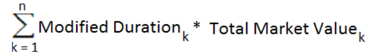
where ‘k’ stands for kth record coming under an Output dimension.

Modified Duration is calculated until the next reprice event. So, if the next reprice event does not fall on the payment event, cash flow on reprice event is used.

§       Dollar Duration (DV01):

The Dollar Duration (DV01) or Present Value of a basis point (PV01) of the instrument is calculated using Modified Duration and Total Market Value.

DV01 is updated back to the instrument table in column DV01_C. Modified Duration and Market value data from the instrument table stored in MODIFIED_DURATION_C and MARKET_VALUE_C is used as input.

For output at the master table (the functional currency), Modified Duration and Market value data from the master table is used.

In detail table (the functional currency) DV01 is populated via FE 721 as follows:

where ‘i’ stands for ith event, and ‘k’ stands for kth record coming under an Output dimension, summed up at each bucket level.

§       Convexity:

The Convexity of the Instrument is calculated as follows:

Where

‘i’ is the ith event, PV is the present value of ith event.

In the master table (the functional currency), the sum of Convexity weighted by Market value, for all records coming under an Output dimension.

§       Average Life

The Average Life of the Instrument is calculated as follows:

§       Yield to Maturity

The Yield to Maturity in OFSAA is the interest rate that equates the present values of the cash flows (coupons & maturity value) to the present Market price.

The YTM takes into account all the sources of income that is:

Coupon interest

Capital Gain or Loss

Reinvestment income - assuming that all the coupons are reinvested at a rate equal to the YTM

The Yield to Maturity is calculated as follows.

The CFE uses the Newton-Rapson method for the calculation of the Yield to Maturity. It starts with the CUR_NET_RATE in the instrument record and iteratively calculates the YTM to a precision of 0.000001. Pseudocode follows:

Step 1:

Initial Value:

Yield to Maturity = Current Net Rate

Delta = 0.0

Total MV = 0

Total Derivative = 0

Step 2:

Loop through each cash flow and calculate Total MV, Total Derivative. At the end of the loop, Delta is calculated. These will be calculated for each iteration.

Conditions for iteration: absolute of Delta > 0.000001 and Iteration > Max Iterations. If Delta goes below 0.000001 or Max Iteration of 500 is reached, iteration stops.

Formula:

v.     Total MV is the summation of MV of each cash flow.

where MV of ith cash flow is calculated as follows:

Where Cash Flows to be used in MV calculation is determined as follows:

If, 'Calculate Market Value' is checked in Process, and

Discount Type = Interest only, then Cash Flow = FE 430.

Discount Type = Principal & Interest, then Cash Flow = FE 210 + FE 430

If 'Calculate Market Value' is checked in Process, and Mature At Reprice option is enabled in Discount Rule, Cash flows till next repricing event is considered. The instrument is assumed to Mature on the next repricing event.

With Discount Type = Interest only, Cash Flow = FE 430 till next Reprice event. If reprice date falls mid-payment, an extra interest till next reprice date is calculated.

With Discount Type = Principal & Interest, then Cash Flow = FE 210 + FE 430 + FE 250. FE 210 for payment events till next reprice events. FE 250 on next reprice events. FE 430 on payment events till the next reprice event. If reprice date falls mid-payment, an extra interest on the next reprice date is calculated.

If the instrument is in Tease, it does not reprice until Tease End Date. See TEASER_END_DATE.

If 'Calculate Market Value' is not checked in the UI: Discount Type = Principal & Interest, then Cash Flow = FE 210 + FE 430.

vi.   Total Derivative is the summation of Derivative of each MV.

where Derivative of ith MV is calculated as follows:

vii.  After a loop through the cash flow ends, the delta is calculated where Total MV and Total Derivative is used.

viii.           

Accrued Interest is calculated as follows.

ICF = First Interest Cash Flow (FE 430).

When Mature At Reprice option is enabled in the Discount Rates interface, and if the first event after as of date, is a Reprice Event (and not in tease), then Accrued Interest is calculated as follows:

ICF is calculated until the next reprice date.

ix.   Yield to Maturity rate is then updated as YTM - Delta.

If engine loops into the next iteration, this updated Yield to Maturity will be used for Total MV and Total Derivative calculation in the next iteration. If there is no further iteration, then updated Yield to maturity will be updated as annualized yield and is output to CUR_YIELD.

And, this YTM Calculated is weighted by CUR_PAR_BAL and written to the RES_MASTER, as = YTM calculated * CUR_PAR_BAL

Step 3:

If absolute of delta > 0.000001 and Max iteration < 500, engine moves to next iteration, and Total MV, Total Derivative, Delta and YTM gets calculated again as mentioned in Step 2.

NOTE:   

Payment per year is calculated as follows:

If Payment Frequency Multiplier is DAY then = 365.0 / Payment Frequency, If Payment Frequency Multiplier is MONTH then = 12.0 / Payment Frequency.

If Payment Frequency Multiplier is YEAR then = 1.0 / Payment Frequency. Where Payment Frequency is data given in PMT_FREQ in Instrument record.

For Payment Schedule records, Payment frequency for a payment date, say date ‘t’, is calculated in Days, as= payment date ‘t’ - payment date just before this specific payment date ‘t-1’. For example, if payment date ‘t’ = 12/15/2017 and ‘t-1’= 11/01/2017, then calculated Payment Frequency = 44 DAYS. As Payment Frequency Multiplier is in DAYs, calculated Payment per Year = 365/44 = 8.29545.

Expired Term is calculated as follows:

When Payment Frequency Multiplier is DAY, then = Cash flow date - As of date.

When Payment Frequency Multiplier is MONTH then = (Cash flow date – As of date) / Days in a month.

Here Days in month= 365/12. When Payment Frequency Multiplier is YEAR then = (Cash flow date - As of date) / 365

§       Effective Interest Rate

The Effective Interest Rate is the true rate of interest earned. The Effective Interest Rate is calculated as follows:

It starts with the CUR_NET_RATE in the instrument record and iteratively calculates EIR to a precision of 0.000001. Pseudocode follows:

Step 1:

Initial Value:

EIR = Current Net Rate

Delta = 0.0

Total MV = 0

Total Derivative = 0

Step 2:

x.     Total MV is the summation of MV of each cash flow.

where MV of ith cash flow is calculated as follows:

Where Cash Flows to be used in MV calculation is determined similarly to the determination of Cash Flows for MV calculation for Yield to Maturity.

xi.   Total Derivative is the summation of Derivative of each MV.

xii.  

where Derivative of ith MV is calculated as follows:

xiii.            After a loop through the cash flow ends, the delta is calculated where Total MV and Total Derivative is used.

Calculation logic of Accrued Interest is detailed in Yield to maturity section.

xiv.           The effective Interest rate is then updated as EIR - Delta.

If the engine loops into the next iteration, this updated Effective Interest rate will be used for Total MV and Total Derivative calculation in the next iteration. If there is no further iteration, then the updated Effective Interest rate is output to EFF_INTEREST_RATE_C.

Step 3:  

If absolute of delta > 0.000001 and Max iteration < 500, engine moves to next iteration, and Total MV, Total Derivative, Delta and EIR gets calculated again as mentioned in Step 2.

Payment per year and Expired Term calculation is detailed in Yield to maturity section.

9.     Update instrument data.

Within the ALM Deterministic Process user interfaces (Static and Dynamic), you can choose to write any of the preceding financial measures for a specified start date back to the instrument table. If this option has been selected, the financial measures are written to the following columns:

The CUR_YIELD column in the instrument record is the annualized yield to maturity of the instrument. It is calculated as follows:

NOTE:   

The difference in output between RES_MASTER and instrument table is that the Instrument table outputs annualized results.

Consolidation of Results

If the Oracle ALM Process optionally specifies Consolidate to Reporting Currency, a cross-currency consolidation is performed. The local currency results are consolidated into a single reporting currency based on the historical and forecast exchange rates. Once translated into the reporting currency, common products are aggregated and output to a set table. For example, if the Process system identifier is uniquely identified by Sys_ID_Num 99999, results would be held as follows:

The currency accounting method determines which exchange rates are used for the translation of each Financial Element. Typically, forecast exchange rates are used for the Temporal and Current Rate methods, and original exchange rates are used for the Historical Basis method. For the Temporal and Current Rate methods, some exceptions apply:

·        Deferred Balances

Deferred balances are balances that reflect prepaid amounts that are prepaid fees, amortized costs, premiums, or discounts. Because the cash flows associated with these balances have already occurred, there is no currency risk associated with them. Therefore, these financial elements are reflected at cost, at the exchange rate at the time of origination.

·        Interest Accruals

The standard historical interest accrual financial element is reflected at the original exchange rate because the currency gain/loss account already reflects the change in interest due to currency. However, to calculate yields consistently with the average balance, a set financial element is calculated for the current basis interest accrual; this reflects the interest accrual based on the current bucket exchange rate.

·        Gap Financial Elements

·        Formula Results

Formula Result output is consolidated into reporting currency using the current bucket exchange rate, irrespective of the currency accounting method selected. Ensure associated currencies are selected for audit, in the ‘Exchange Rate’ section within the ‘Audit’ block of a process.

If respective currencies are not selected for audit, or if the audit is disabled, the engine will use the actual exchange rate on As of date for consolidation.

NOTE:   

The formula result output is consolidated using the current bucket exchange rate. Whereas Static and Dynamic Business output is consolidated using currency accounting method and financial elements. For more information, see the Currency Translation Methods for Financial Elements.

Hence, the formula result in consolidated output, and Static/Dynamic business consolidated output may vary.

For Consolidated Master results: Deferred balances are translated using the exchange rate in effect when the instrument was originated; all other balances are translated using the exchange rate in effect at the As-of-Date or future Start Date:

·        As-of-Date values use the actual exchange rate in effect on the As-of-Date.

·        Future originations and Dynamic Start Date values respectively use the forecast exchange rate in effect on the future origination date or Start Date.

If no exchange rate is found, the cash flow engine logs an error message and sets the exchange rate equal to 1.

Currency-Based Gap Modeling

The processing steps depend on the relationship between the gap and cash flow modeling buckets. Because modeling buckets may differ between the cash flow results and the gap results and exchange rate forecasts are defined for cash flow modeling buckets only, additional processing steps are employed when there are bucket differences.

·        Compatible (consistent) gap and cash flow buckets

If cash flow modeling buckets and gap buckets are equal, or if multiple gap modeling buckets can even fit into one cash flow modeling bucket, the forecast exchange rates for the cash flow modeling buckets are used.

·        Unevenly-Overlapping gap and cash flow buckets

If cash flow modeling buckets are smaller than gap modeling buckets or if their respective start and end dates do not coincide, the engine must derive the forecast exchange rates for the gap modeling buckets.

In this special case, the cash flow engine calculates a time-weighted exchange rate forecast for the gap bucket. Bear in mind that with a time-weighted rate, the consolidated gap results may be different than the consolidated cash flow results, even though they came from the same local balance. For example, a cash flow of $10 at an exchange rate of 1 and cash flow of $20 at an exchange rate of 2 sums up to a translated cash flow of 20 (10 divided by 1, plus 20 divided by 2). If the weighted-average exchange rate is calculated as 1.5, the translated cash flow equals 20 (10 plus 20, divided by 1.5).

We recommend that consistent modeling and gap buckets be used in multicurrency simulations, to eliminate potential data inconsistency issues.

Detail Cash Flow Data

Event Use Code Values

I = Initialization of record

P = Payment

PC = Payment Recalculation

PP = Prepayment

R = Reprice

D = Deferred amortization

Rule of 78's Example

Example: 12 month loan with current payment of $93.33 and original balance = $1,000.00

1.     Sum all principal and interest payments made over the life of the instrument:

cash flow= current payment * total number of payments

= $93.33 * 12

= $1,120.00

2.     Determine total amount of interest paid over the life of the instrument:

interest= cash flow - original par balance

= $1,120.00 - $1,000.00

= $120.00

3.     Sum the payment numbers.

pmts= total no. payments * (total no. payments + 1)/2

= 12 * 13/2

= 78

4.     Calculate principal and interest amount at each payment.

interest=interest * (payments remaining/ pmts)

principal= current payment - interest

Volatility Surface Calculation

When you have defined a Forecast Rates and assigned the percentage shock amount to one or more rate scenarios, then the following formula is used for target ALM surface:

Target ALM Surface = (1+(SHOCK_AMT/100))*ALM_Vol

Where:

SHOCK_AMT is the specified value from FSI_FCAST_ALMVOL

ALM_Vol are all values from the target ALM Surface matrix (FSI_IRC_VOL_SURFACE_RATE_HIST)

Examples:

·        ALM Vol Surface Shock Calculations

For example, if there are no shocks applied, that is following base ALM vol surface with original values:

If you have specified a value of 1 as the percentage shock for Scenario One, then FSI_FCAST_ALMVOL. SHOCK_AMT = 1

In the subsequent forecast for Black 76 embedded option valuation, the Application will apply this percentage to all values in the matrix.For example, for Strike 2, the initial value was 25% (on 12/31/2010) and the up shock of 1% would be calculated as:

(1+(1/100))*25 = 25.25

This calculation is repeated for every remaining volatility entry, as shown:

·        After 1% Up Shock:

The same procedure is repeated if the shock scenario were a negative amount, for example, -1% shock amount. The formula would be: (1+(-1/100))*25 = 25.25

NOTE:   

The shock amounts are always applied to the Base scenario. This process is repeated for all remaining volatilities, as displayed

·        After 1% DOWN Shock:

The ALM volatilities are stored isFSI_IRC_VOL_SURFACE_RATE_HIST. When a user defines an ALM Shock, it is joined to this table by INTEREST_RATE_CD. An ALM Vol Surface can have multiple effective dates but this is irrelevant until processing occurs as only one As-of Date is selected in a process.

·        INTEREST_RATE_CD: defines the ALM Vol surface unique code

·        EFFECTIVE_DATE: The effective date of the ALM Vol. This should match the As-of Date in a process.

·        EXPIRAITON_DATE: Nominal date dimension for ALM Vol (horizontal)

·        VOL_SURFACE_STRIKE: The nominal strike value dimension (vertical)

·        VOLATILITY: Numerical volatility percent (that is 40 is interpreted as 40%). This is the amount that is shocked when users define a shocking percentage in FSI_FCAST_ALMVOL. SHOCK_AMT. This new shocking amount is the new volatility that is applied in Black 76 option value calculations for every scenario in the forecast.

Example:

·        If there is a qualified existing ALM Vol Surface defined in FSI_IRC_VOL_SURFACE_RATE_HIST, as follows:

·        The table FSI_FCAST_ALMVOL is populated as follows:

Thus, in a forecast for Scenario A, all ALM vols would receive a 1% shock using the definition above. This is repeated for every scenario (A, B, and C) in the FCR definition for the process forecast.

Execution Logs

Case Flow Engine logs (.log and .err) file used to get generated under $FIC_DB_HOME/log/FusionApps.

From v8.0.6.0.0 onwards, the logs are generated in the following folder locations:

Figure 2: Folder Structure of Execution Logs

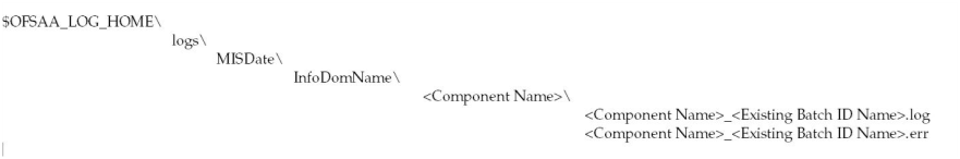
NOTE:   

Here, <Component Name> maps to V_COMPONENT_ID from COMPONENT_MASTER table for specific V_PROG_ID where V_PROG_ID represent App Specific executable name.

To achieve this, follow these steps:

1.     The installer provides a new environment variable OFSAA_LOG_HOME that points to FTPSHARE/logs folder’s location.

2.     Engine reads$OFSAA_LOG_HOME value to find the location of the log and creates the folder structure in the following order, if not present.

For example:

Figure: Folder Structure Example of Execution Logs

The log file name is prefixed with the Component name (mentioned above) instead of prefixing the log file name with “<executable>.”

Entry is available in the “.ini” file (e.g. for ALM its ofsrm.ini) named “ComponentName” which is configurable and initially set the same present in COMOPNENT_MASTER table for the respective application. Add this entry in .ini file if it is not available.

NOTE:   

You can make some changes in the .ini file to improve the cash flow engine performance.

Add CursorSharingMode entry in .ini file.

Engine reads the value against Key CursorSharingMode and sets CURSOR_SHARE at the DB Session level accordingly.

The engine executes the following statement if the value set against CursorSharingMode Key.

ALTER SESSION SET CURSOR_SHARING = <Input Value> in upper case

<Input Values>: EXACT, FORCE, SIMILAR

If the value is not supplied, then Engine would NOT set any alter statement.

In case of upgrade path, installer takes care of renaming CFE artifacts (log files/folders) from Cash Flow Engine to Asset Liability Management. This allows you to view existing engine log files (generated during 8.1) from View Logger.