13 The Oracle Funds Transfer Pricing Process

Oracle Funds Transfer Pricing (FTP) application is based on the Oracle Financial Services Analytical Applications Infrastructure (OFSAAI). OFSAAI is the central, integrated data source on which Oracle Financial Services Analytical (OFSAA) applications are built. This description of the Oracle Funds Transfer Pricing process assumes that your system administrator has set up the OFSAAI data repository and has populated it with your enterprise-wide business data. For more information, see the Oracle Financial Services Analytical Applications Infrastructure User Guide.

Oracle Funds Transfer Pricing allows you to transfer price instruments, such as mortgages and commercial loans, stored in your Instrument tables, as well as aggregated information, such as cash and other assets, and equity, residing in the Management Ledger table.

Consequently, while transfer pricing you need to select the Account tables as the data source for instruments and the Management Ledger Table for aggregated information.

The Oracle Funds Transfer Pricing process comprises the following steps:

·        Reconciling the data

·        Cleansing the data by Performing Cash Flow Edits

·        Setting Application Preferences

·        Capturing instrument behavior by

·        Defining Behavior Patterns

·        Defining Payment Patterns

·        Defining Repricing Patterns

·        Activating Currencies and loading exchange rates

·        (Mandatory) Deciding on historical rate information and managing it by Creating Interest Rate Codes

·        Setting Stochastic Rate Index Rules

·        (Mandatory) Defining Transfer Pricing Rules

·        Setting Prepayment Model Rules

·        Defining Prepayment Rules

·        Defining Adjustment Rules

·        Defining Alternate Rate Output Mapping Rules

·        Creating a Propagation Pattern

·        (Mandatory) Defining and Executing the Transfer Pricing Process

·        Reviewing processing errors

·        Accessing Transfer Pricing, Detail Cash Flow Results for Audit Purposes

·        Accessing Transfer Pricing, Interest Rate Audit Results

·        Analyzing results

·        Reprocessing erroneous accounts

Topics:

·        Define Transfer Pricing Rules

·        Transfer Pricing Methodologies and Rules

·        Define Prepayment Rules

·        Define Adjustment Rules

·        Define Alternate Rate Output Mapping Rules

·        Define and Execute a Transfer Pricing Process

·        Define and Execute a Break Identification Process

·        The Ledger Migration Process

·        Define Behavior Patterns

·        Define Payment Patterns

·        Define Repricing Patterns

·        Perform Cash Flow Edits

·        Create Interest Rate Codes

·        Access Transfer Pricing Detail Cash Flow Results for Audit Purposes

·        Access Transfer Pricing Interest Rate Audit Results

·        Analyze Results

·        Review Processing Errors

·        Reprocess Erroneous Accounts

·        Reconcile the Data

Define Transfer Pricing Rules

Defining Transfer Pricing rules is one of the mandatory steps in the Oracle Funds Transfer Pricing process. You must define Transfer Pricing rules, to transfer price your products. A Transfer Pricing rule is used to manage the association of transfer pricing methodologies to various product-currency combinations. It can also be used to manage certain parameters used in option costing.

To reduce the amount of effort required to define the transfer pricing methodologies for various products and currencies, Oracle Funds Transfer Pricing allows you to define transfer pricing methodologies using node level and conditional assumptions.

·        Node Level Assumptions: Oracle Funds Transfer Pricing uses the Product Dimension that has been selected within Application Preferences, to represent a financial institution's product port­folio. Using this dimension, you can organize your product portfolio into a hierarchical structure and define parent-child relationships for different nodes of your product hierarchy. This signifi­cantly reduces the amount of work required to define transfer pricing, prepayment, and adjust­ment rule methodologies.

·        You can define transfer pricing, prepayment, and adjustment rule methodologies at any level of your product hierarchy. Children of parent nodes on a hierarchy automatically inherit the meth­odologies defined for the parent nodes. However, methodologies directly defined for a child take precedence over those at the parent level. For more information, see Defining Transfer Pricing Methodologies Using Node Level Assumptions.

·        Conditional Assumptions: The conditional assumption feature allows you to segregate your product portfolio based on common characteristics, such as term to maturity, origination date, and repricing frequency, and assign specific transfer pricing methodologies to each of the groupings.

For example, you can slice a portfolio of commercial loans based on repricing characteristics and assign one global set of Transfer Pricing, Prepayment, or Adjustment rule methods to the fixed-rate loans and another to the floating-rate loans. For more information, see Associating Conditional Assumptions with Assumption Rules.

Transfer Pricing Methodologies and Rules

The transfer pricing methodologies supported by Oracle Funds Transfer Pricing can be grouped into the following categories:

Cash Flow Transfer Pricing Methods: Cash flow transfer pricing methods are used to transfer price instruments that amortize over time. They generate transfer rates based on the cash flow characteristics of the instruments.

To generate cash flows, the system requires a detailed set of transaction-level data attributes, such as, origination date, outstanding balance, contracted rate, and maturity date, which resides only in the Instrument tables. Consequently, cash flow methods apply only if the data source is Account tables. Data stored in the Management Ledger Table reflects only accounting entry positions at a particular point in time and does not have the required financial details to generate cash flows, thus preventing you from applying cash flow methodologies to this data.

The cash flow methods are also unique in that Prepayment rules are used only with these methods. You can select the required Prepayment rule when defining a Transfer Pricing Process.

Oracle Funds Transfer Pricing supports the following cash flow transfer pricing methods:

·        Cash Flow: Average Life

·        Cash Flow: Duration

·        Cash Flow: Weighted Term

·        Cash Flow: Zero Discount Factors

Non-cash Flow Transfer Pricing Methods: These methods do not require the calculation of cash flows. While some of the non-cash flow methods are available only with the Account tables data source, some are available with both the Account and Ledger table data sources.

Oracle Funds Transfer Pricing supports the following non-cash flow transfer pricing methods:

·        Moving Averages

·        Straight Term

·        Spread from Interest Rate Code

·        Spread from Note Rate

·        Redemption Curve

·        Tractor Method

·        Caterpillar

·        Weighted Average Perpetual

·        Unpriced Account

Oracle Funds Transfer Pricing also allows Mid-period Repricing. This option allows you to take into account the impact of high market rate volatility while generating transfer prices for your products. However, the mid-period repricing option applies only to adjustable-rate instruments and is available only for certain non-cash flow transfer pricing methods.

Note on Bulk Updates versus Row by Row Processing: Any TP method that does not refer to individual account characteristics utilizes a bulk update to assign a single transfer rate to a group of instrument records. Any TP Method that needs to refer to individual account characteristics to process will execute on a row by row basis. In general, Bulk updates will be faster than row by row processing.

The following TP methods, when not defined through a conditional assumption and not utilizing Mid-Period Repricing, use Bulk Updates:

·        Redemption Curve (Assignment Date = As of Date only)

·        Moving Average

·        Spread from Note Rate

·        Spread from IRC (Assignment Date = As of Date only)

·        Tractor

·        Caterpillar

·        Weighted Average Perpetual

All other TP Methods are processed row-by-row. When Conditional Assumptions or Mid Period Repricing are used, processing will always be row-by-row, regardless of the TP Method selection.

Cash Flow: Average Life

The Average Life method determines the average life of the instrument by calculating the effective term required to repay half of the principal or nominal amount of the instrument. The TP rate is equivalent to the rate on the associated interest rate curve corresponding to the calculated term.

Oracle Funds Transfer Pricing derives the Average Life based on the cash flows of an instrument as determined by the characteristics specified in the Instrument Table and using your specified prepayment rate, if applicable. The average life formula calculates a single term, that is, a point on the yield curve used to transfer price the instrument being analyzed. The Average Life calculation does not differentiate between fixed-rate and adjustable-rate instruments. It applies the same calculation logic to both. i.e. it computes the Average Life of the loan (to maturity).

Users also have the choice to populate the TP_AVERAGE_LIFE column directly with a value computed outside of OFSAA FTP. If this value is populated, the FTP engine will read the TP_AVERAGE_LIFE and will lookup the FTP rate for the given term. In this case, the TP Engine will not generate cash flows and will not re-compute the Average Life. It will simply use the value that has been provided and look up the appropriate FTP rate from the specified TP Interest Rate Curve.

Cash Flow: Duration

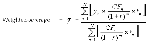
The Duration method uses the Macaulay duration formula:

In this formula:

·        N: Total number of payments from Start Date until the earlier of repricing or maturity

·        CFn: Cash flow (such as regular principal, prepayments, and interest) in period n

·        r: Periodic rate (current rate/payments per year)

·        m: Remaining term to cash flow/active payment frequency

·        tn: Remaining term to cash flow n, expressed in years

Oracle Funds Transfer Pricing derives the Macaulay duration based on the cash flows of an instrument as determined by the characteristics specified in the Instrument Table and using your specified prepayment rate, if applicable. The duration formula calculates a single term, that is, a point on the yield curve used to transfer price the instrument.

·        Within the Duration calculation, the discount rate or current rate, r, is defined in one of three ways, based on how the methodology is set up by the user:

§        The current rate is defined as the current net rate if the processing option, "Model with Gross Rates" is not selected and the current gross rate if the option is selected. The current rate is used as a constant discount rate for each cash flow.

§        The user may directly input while defining the TP rule, a constant rate to use for discounts. If specified, this rate is used as a constant discount rate for each flow.

§        The user can select to discount the cash flows using spot rates from a selected interest rate curve. With this approach, a discount rate is read from the selected interest rate curve corre­sponding to the term of each cash flow.

Users also have the choice to populate the TP_DURATION column directly with a value computed outside of OFSAA FTP. If this value is populated, the FTP engine will read the TP_DURATION and will lookup the FTP rate for the given term. In this case, the TP Engine will not generate cash flows and will not re-compute the DURATION. It will simply use the value that has been provided and look up the appropriate FTP rate from the specified TP Interest Rate Curve.

Cash Flow: Weighted Term

The Weighted Term method builds on the theoretical concepts of duration. You can use the Cash flow Duration TP method approach to the Cash flow Weighted Term method. Based on that, following two Cash Flow Discounting Methods are used:

·        Multiple Rate

·        Single Rate

For more information, see the Transfer Pricing Rules section.

As shown earlier, duration calculates a weighted-average term by weighting each period, n, with the present value of the cash flow (discounted by the rate on the instrument) in that period.

Since the goal of the Weighted Term method is to calculate a weighted average transfer rate, it weights the transfer rate in each period, yn, by the present value for the cash flow of that period. Furthermore, the transfer rates are weighted by an additional component, time, to account for the length of time over which a transfer rate is applicable. The time component accounts for the relative significance of each strip cash flow to the total transfer pricing interest income/expense. The total transfer pricing interest income/expense on any cash flow is a product of that cash flow, the transfer rate, and the term. Hence, long-term cash flows will have a relatively larger impact on the average transfer rate. The Weighted Term method, with "Discounted Cash Flow" option selected, can be summarized by the following formula:

In this formula:

·        N: Total number of payments from Start Date until the earlier of repricing or maturity

·        CFn: Cash flow (such as regular principal, prepayments, and interest) in period n

·        r: Periodic rate (current rate/payments per year)

·        m: Remaining term to cash flow n/active payment frequency

·        tn: Remaining term to cash flow n, expressed in years

·        yn: Transfer rate in period n

Within the Cash Flow Weighted Term method definition screen, users can select the Cash flow type as either Principal + Interest (the default selection) or Principal Only. This selection will impact the CFn in the above formula.

Additionally, users can choose whether or not to discount the cash flows as described above. If the "Cash Flow" option is selected rather than "Discounted Cash Flow", the following simplified formula is applied:

The discount rate or current rate, r, is defined in one of three ways, based on how the methodology is set up by the user:

·        The current rate is defined as the current net rate from the instrument record unless the pro­cessing option, "Model with Gross Rates" is selected, in which case, the current gross rate is used. The current rate is used as a constant discount rate for each cash flow.

·        The user may directly input while defining the TP rule, a single constant rate to use for discounts. If specified, this rate is used as a constant discount rate for each cash flow.

·        The user can select to discount the cash flows using spot rates from a selected interest rate curve. With this approach, a discount rate is read from the selected interest rate curve corre­sponding to the term of each cash flow.

Cash Flow: Zero Discount Factors

The Zero Discount Factors (ZDF) method takes into account common market practices in valuing fixed-rate amortizing instruments. For example, all Treasury strips are quoted as discount factors. A discount factor represents the amount paid today to receive $1 at maturity date with no intervening cash flows (that is, zero-coupons).

The Treasury discount factor for any maturity (as well as all other rates quoted in the market) is always a function of the discount factors with shorter maturities. This ensures that no risk-free arbitrage exists in the market. Based on this concept, one can conclude that the rate quoted for fixed-rate amortizing instruments is also a combination of some set of market discount factors. Discounting the monthly cash flows for that instrument (calculated based on the constant instrument rate) by the market discount factors generates the par value of that instrument (otherwise there is arbitrage).

ZDF starts with the assertion that an institution tries to find a funding source that has the same principal repayment factor as the instrument being funded. In essence, the institution strip funds each principal flow using its funding curve (that is, the transfer pricing yield curve). The difference between the interest flows from the instrument and its funding source is the net income from that instrument.

Next, ZDF tries to ensure consistency between the original balance of the instrument and the amount of funding required at origination. Based on the transfer pricing yield used to fund the instrument, the ZDF solves for a single transfer rate that would amortize the funding in two ways:

Its principal flows match those of the instrument.

The Present Value (PV) of the funding cash flows (that is, the original balance) matches the original balance of the instrument.

ZDF uses zero-coupon factors (derived from the original transfer rates, see the example below) because they are the appropriate vehicles in strip funding (that is, there are no intermediate cash flows between origination date and the date the particular cash flow is received). The zero-coupon yield curve can be universally applied to all kinds of instruments.

This approach yields the following formula to solve for a weighted average transfer rate based on the payment dates derived from the instrument's payment data.

Zero Discount Factors = y =

In this formula:

·        B₀: Beginning balance at the time, 0

·        B_n-1: Ending balance in the previous period

·        B_n: Ending balance in the current period

·        DTP_n: Discount factor in period n based on the TP yield curve

·        N: Total number of payments from Start Date until the earlier of repricing or maturity

·        p: Payments per year based on the payment frequency; (for example, monthly payments gives p=12)

Deriving Zero-Coupon Discount Factors: An Example

This table illustrates how to derive zero coupon discount factors from monthly pay transfer pricing rates:

Moving Averages

Under this method, a user-definable moving average of any point on the transfer pricing yield curve can be applied to a transaction record to generate transfer prices. For example, you can use a 12-month moving average of the 12-month rate to transfer price a particular product.

The following options become available on the user interface (UI) with this method:

·        Interest Rate Code: Select the Interest Rate Code to be used as the yield curve to generate trans­fer rates.

·        Yield Curve Term: The Yield Curve Term defines the point on the Interest Rate Code that is used.

·        Historical Range: The Historical Term defines the period over which the average is calculated.

The following table illustrates the difference between the yield curve and historical terms.      

The range of dates is based on the As of date minus the historical term plus one, because the historical term includes the As of date. Oracle Funds Transfer Pricing takes the values of the yield curve points that fall within that range and does a straight average on them.

For example, if As of Date is Nov 21, the Yield Curve Term selected is Daily, and the Historical Term selected is 3 Days, then, the system will calculate the three-day moving average based on the rates for Nov 19, 20, and 21. The same logic applies to monthly or annual yield terms.

Straight Term

When you select the Straight Term method and standard Term approach, the system derives the transfer rate using the last repricing date and the next repricing date for adjustable rate instruments, and the origination date and the maturity date for fixed-rate instruments.

·        Standard Calculation Mode:

§        For Fixed Rate Products (Repricing Frequency = 0), use Yield Curve Date = Origination Date, Yield Curve Term = Maturity Date-Origination Date.

§        For Adjustable Rate Products (Repricing Frequency > 0)

—     For loans still in the tease period (tease end date > As of Date, and tease end date > origination date), use Origination Date and Tease End Date - Origination Date.

—     For loans not in the tease period, use Last Repricing Date and Repricing Frequency.

·        Remaining Term Calculation Mode:

§        For Fixed Rate Products, use As of Date and Maturity - As of Date.

§        For Adjustable Rate Products, use As of Date and Next Repricing Date - As of Date.

In addition to the above standard logic used for determining the appropriate “Term”, users also have the option to select either Original Term or Repricing Frequency and also have the option to modify these terms using simple mathematical operators. These options can be useful in cases where the straight term method needs to be applied to the same record under different circumstances. For example, for calculating the base rate on an adjustable rate instrument, the standard approach should be used. For the same instrument, users may further want to use the entire original term for applying a liquidity premium or other add-on rate. To support the second case, we give the option to directly specify the term to be used, and we further provide the option to modify the term using simple operators, such as +, -, *, /.

The following options become available in the application with this method:

·        Term: Select from Standard, Original Term, or Reprice Frequency. Standard is the default selec­tion and the resulting Term will follow the above logic. The Original Term and Reprice Frequency options allow users to override the standard logic and specify which term to use.

·        Adjustment Operator: When either Original Term or Reprice Frequency is selected as the Term, the Adjustment Operator becomes active. The term adjustment is optional and gives users the ability to modify the term

·        Adjustment Amount: This input works together with the adjustment operator to indicate how the term should be modified

·        Interest Rate Code: Select the Interest Rate Code to be used for transfer pricing the account.

·        Mid-Period Repricing Option: Select the check box beside this option to invoke the Mid-Period Repricing option.

·        Holiday Calendar: Select if a holiday calendar is applicable for calculating the charges/credits or for calculating Economic Value

·        Rolling Convention: Select the appropriate business day rolling convention if a Holiday Calen­dar is selected

·        Interest Calculation logic: Select the appropriate option to indicate how the interest payment should be adjusted when a holiday date is encountered

For more information, see the Transfer Pricing Rules chapter.

Spread from Interest Rate Code

Under this method, the transfer rate is determined as a fixed spread from any point on an Interest Rate Code. The following options become available on the application with this method:

·        Interest Rate Code: Select the Interest Rate Code for transfer pricing the account.

·        Yield Curve Term: The Yield Curve Term defines the point on the Interest Rate Code that will be used to transfer price. If the Interest Rate Code is a single rate, the Yield Curve Term is irrelevant. Select Days, Months, or Years from the drop-down list, and enter the number.

·        Lag Term: While using a yield curve from an earlier date than the Assignment Date, you need to assign the Lag Term to specify a length of time before the Assignment Date.

·        Rate Spread: The transfer rate is a fixed spread from the rate on the transfer rate yield curve. The Rate Spread field allows you to specify this spread.

·        Assignment Date: The Assignment Date allows you to choose the date for which the yield curve values are to be picked up. Choices available are the As of Date, Last Repricing Date, Origination Date, or TP Effective Date.

·        Mid-Period Repricing Option: Select the check box beside this option to invoke the Mid-Period Repricing option.

Spread from Note Rate

To generate transfer prices using this method, you need to provide just one parameter: a rate spread. This spread is added or subtracted from the coupon rate of the underlying transaction to generate the final transfer rate for that record.

While entering the rate spread, make sure to input it with the appropriately positive or negative sign, as illustrated in the following table. The first row describes a situation where you are transfer pricing an asset and want to have a positive matched spread for it (the difference between the contractual rate of the transaction and the transfer rate is positive). Here, you need to enter a negative rate spread.

The following option becomes available in the application when you select this method:

·        Mid-Period Repricing Option: Select the check box beside this option to invoke the Mid-Period Repricing option.

Redemption Curve

This method allows you to select multiple-term points from your transfer pricing yield curve and calculate an average transfer rate based on the weights you assign to each term point. The following options become available in the application with this method:

·        Interest Rate Code: Select the Interest Rate Code which you want to use as the transfer pricing yield curve.

·        Assignment Date: The Assignment Date allows you to choose the date for which the yield curve values will be picked up. Choices available are the As of Date, Last Repricing Date, Origination Date, or TP Effective Date.

·        Percentages/Term Points: See Redemption Curve

·        Mid-Period Repricing Option: Select the check box beside this option to invoke the Mid-Period Repricing option.

Tractor Method

The Tractor Method extends the concept of “Strip Funding” to instruments that do not have contractual cash flows. These products are known as perpetual or non-maturity products and hence do not generate contractual cash flows. The process of determining transfer rates requires adopting the strip funding approach by splitting these products into Core and Volatile portions based on statistically established Behavioral Profiles. With this method, the volatile portion is considered to have an overnight maturity and the core portion is assigned a longer maturity (through a Behavior Pattern) which is comprised of a series of balance strips corresponding to the maximum tenor of the portfolio (on the origination of the portfolio, original strips will have shorter maturities). Each strip is assigned a transfer rate corresponding to its origination date and corresponding term. The historical, active strips are retained for the portfolio and the portfolio transfer rate is determined based on the weighted average transfer rate of the strips comprising the portfolio. The weighted average rate from the strip portfolio is written back to all instrument records that are mapped to this portfolio through the Transfer Pricing rule.

The characteristics of the replicating portfolio used by the Tractor Method are defined through a Non-Maturity Behavior Pattern with replicating portfolio options. The following example illustrates the behavior of a small 3-day portfolio rolling across 4 days.

Replicating Portfolio                  

The above example assumes a business day calendar is enabled with the following business days defined:

·        Business Day

·        Calendar

·        31-Jan-11

·        1-Feb-11

·        2-Feb-11

·        3-Feb-11

·        4-Feb-11

·        7-Feb-11

·        8-Feb-11

·        9-Feb-11

·        10-Feb-11

·        11-Feb-11

Caterpillar

The Caterpillar method extends the concept of “strip funding” to instruments that do not have contractual cash flows. These products are known as Perpetual or Non-Maturity Products and hence do not generate contractual cash flows. The process of determining Transfer Rates requires adopting the 'Strip Funding Approach' by splitting these products into 'Core' and 'Volatile' portions based on statistically established Behavioral Profiles. With this approach, the volatile portion may be considered as an overnight funding strip and the core portion can be dealt with by an assumed maturity structure defined through a Behavior Pattern. For example, statistical analysis may imply that the Savings Account portfolio behaves 20% as volatile and 80% as the core of which the maturity is likely to be 3 months. Hence the Funding Strips that would get created are 20% 1 month, and 80% 3 months.                        

In the above example, we assume that once a funding strip is assigned a certain Transfer Rate based on its original term, the rate remains constant until the strip matures. Each strip is funded for the original term based on the yield curve in effect at the start of the strip. In month 4, when the balance is 9000, the strips still outstanding from earlier months are 3040 as a 3-month term strip, created in month 2 at 5% having a remaining term 1-month; (3870-3040) 1-month term strip created in month 4, 1808 3-month term strip created in month 3 with 2-month remaining term, and 3322 3-month term strip created in month 4. The weighted average rate of these strips comes to 5.52% as illustrated in the example above.

In summary:

Month 4 Transfer Rate = (3040*5% + (3870-3040)*5.5% + 1808*5.5% + 3322*6%) / 9000 = 5.52%

Weighted Average Perpetual

This method calculates the simple weighted average of the applicable balance based on maturity bands defined through a Behavior Pattern. In the following example, the end of period balance as of Jan 31 is split into Core and Volatile strips and the relevant rates are applied to arrive at the weighted average Transfer Rate.

Transfer Rate = (20000*3.10% + 80000*3.50%) / 100000 = 3.42%

·        Behavior Pattern: Select the Behavior Pattern that is associated with the Product / Currency combination being defined.

·        Interest Rate Code: Select the Interest Rate Code which you want to use as the transfer pricing yield curve.

Unpriced Account

Under the unpriced account method, the transfer rate for the account is defined as the weighted average of the Product dimension members. While using the unpriced account methodology, you can specify whether the weighted average of transfer rates has to be taken across all organizational units or for accounts only within that organizational unit.

The following options become available in the application with this method:

·        Add Dimension Values: Allows you to select the Product dimension members whose weighted average transfer rate will be assigned to the product being defined.

·        Across all Organization Units: Allows you to specify whether the weighted average of transfer rates should be taken across all organizational units. If this option is not selected, the weighted average rate will be calculated for each org unit. To calculate for each individual Org Unit, you must also select the Org Unit dimension under Migration Dimensions in the Transfer Pricing Process.

Transfer Pricing Methods and the Mid-Period Repricing Option

The mid-period repricing option allows you to take into account the impact of high market rate volatility while generating transfer rates for your products. However, the mid-period repricing option applies only to adjustable rate instruments and is available only for the following non-cash flow transfer pricing methods:

·        Straight Term

·        Spread from Interest Rate Code

·        Spread from Note Rate

·        Redemption Curve

The rationale behind mid-period repricing is as follows. If you do not select the Mid-Period Repricing option, Oracle Funds Transfer Pricing computes the transfer rate for an adjustable-rate instrument based upon its last repricing date. The assumption behind this method of calculation is that the input transfer rate for a month should be the daily average transfer rate for that entire month. Consequently, all instruments repricing in that month derive their transfer rates from the same (average) transfer pricing yield curve. However, this approach misstates the transfer rate, in periods when the interest rate level has moved substantially since the last repricing.

Take the example of a one-year adjustable-rate loan. Suppose it reprices on the 15th of the month, and that transfer rates have moved up 200 basis points since the last reprice. In such a case, the theoretically pure transfer rate for the first half of the month should be 200 basis points lower than the transfer rate for the second half of the month. To apply such theoretical accuracy to your transfer pricing results, you should select the Mid-Period Repricing option.

Mid-Period Repricing Computations:

The Mid-Period Repricing option uses two columns in the Instrument Tables (Current- and Prior- Repricing Period Average Daily Balance: CUR_TP_PER_ADB, PRIOR_TP_PER_ADB) that are exclusively devoted to this option. These columns must be accurately populated for the Mid-Period Repricing results to be accurate.

The Mid-Period Repricing Computation process comprises the following steps:

1.       Computation of transfer rate for the current repricing period.

2.      If the computed last repricing date > beginning of processing month, roll back to prior repricing date.

3.      Computation of prior period transfer rate.

4.     Repetition of steps 2 and 3 as necessary.

5.      Computation of the final transfer rate by weighting the results (from current and previous repricing periods) by average balances and days.

6.     Application of the final transfer rate to the instrument record.

Typical Calculations

The following diagram depicts a typical Mid-Period Repricing situation where the instrument reprices during the current processing month.

Figure 1:   Mid-Period Repricing

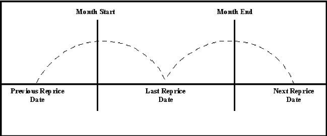
If an instrument reprices during the current processing month, then there are multiple repricing periods spanning the current month. In this example, there are two repricing periods in the current processing month and the computed last repricing date > beginning of processing month. Consequently, the repricing dates need to be rolled back by the repricing frequency until the Prior Last Repricing Date (Prior LRD) <= Beginning of Month and the Mid-Period Repricing Computation process should be executed as follows:

·        Computation of transfer rate for the current repricing period.

§        Transfer Pricing Term: Next Reprice Date - Last Reprice Date

§        Transfer Pricing Date: Last Reprice Date

§        Number of Days at that Rate: End of Month + 1- Last Reprice Date

If the Computed Next Reprice Date (the next repricing date for a given repricing period) is less than or equal to the End of Month, then the Number of Days calculation uses the Computed Next Reprice Date in place of End of Month. In other words, the Number of Days equals the Minimum (End of Month + 1, Computed Next Reprice Date) - Maximum (Beginning of Month, Computed Last Reprice Date). This example assumes the use of the Straight Term transfer pricing method. The following table describes the logic for the computation of the transfer rates for each method.

·        If the computed last repricing date > beginning of processing month, roll back to prior repricing date.

Since the Last Repricing Date is greater than the Beginning of the Processing month, the Roll Back is done as follows:

Computed Next Reprice Date is reset to Last Reprice Date

Computed Last Repricing Date is reset to Last Repricing Date - Reprice Frequency (Prior LRD)

·        Computation of the prior period transfer rate.

§        Transfer Pricing Term: Last Reprice Date - Prior LRD

§        Transfer Pricing Date: Prior LRD

§        Number of Days at that Rate: Last Reprice Date - Beginning of Month

If the Computed Last Reprice Date (the last repricing date for a given repricing period) is greater than the Beginning of Month, then the Number of Days calculation uses Computed Last Reprice Date in place of the Beginning of Month. In other words, the Number of Days equals Minimum (End of Month + 1, Computed Next Reprice Date) - Maximum (Beginning of Month, Computed Last Reprice Date).

§        Repetition of steps 2 and 3 as necessary. In this example, only one iteration is needed because Prior LRD is less than the Beginning of the Month.

§        Computation of the final transfer rate by weighting the results (from current and previous repricing periods) by average balances and days.

The calculation makes the following assumptions:

·        CUR_TP_PER_ADB is the balance applying since the last reprice date

·        PRIOR_TP_PER_ADB is the balance applying to all prior repricing periods

·        Application of the final transfer rate to the instrument record.

Exceptions to Typical Calculations

There are two exceptions to typical mid-period repricing computations:

·        Teased Loan Exception: When the TEASER_END_DATE is the first repricing date, it overrides all other values for LAST_REPRICE_DATE and NEXT_REPRICE_DATE. During the Teased Period, then, the Computed Last Repricing Date equals the Origination Date and the Computed Next Reprice Date equals the TEASER_END_DATE. Consequently:

§        If the TEASER_END_DATE is greater than the AS_OF_DATE, the Mid-Period Repricing does not apply. The logic to compute the Transfer rate is based upon the term equal to the TEAS­ER_END_DATE - ORIGINATION_DATE, date equals the ORIGINATION_DATE.

§        When rolling backward by repricing frequency, if the TEASER_END_DATE is greater than the Computed Last Repricing Date, Transfer Pricing computes the transfer rates for that period based on the teased loan exception.

·        Origination Date Exception: While performing mid-period repricing computations, Oracle Funds Transfer Pricing assumes that if the origination date occurs during the processing month, the calculation of the number of days (used for weighting) originates on the first day of the month. This is a safe assumption because the PRIOR_TP_PER_ADB value shows this instrument was not on the books for the entire month. This impact is measured because the PRIOR_T­P_PER_ADB value is used in computing the weighted average transfer rate. If Oracle Funds Transfer Pricing were to shorten the number of days (as in the weighted average calculation), it would double-count the impact.

Origination Date Exception: An Example

The following table displays a situation where the origination date occurs during the processing month:

Taking the origination date exception into account, the Mid-Period Repricing calculation is done as follows:

(6% * $50 * 20 days) + (8% * $100 * 10 days) / ($50 * 20 days + $100 * 10 days) = 7%

If period 1 was not taken into account, the result would have been, (6% * $50 * 10 days) + (8% * $100 * 10 days) / ($50 * 10 days + $100 * 10 days) = 7.33%, which is incorrect.

Defining Transfer Pricing Methodologies Using Node Level Assumptions

In Oracle Funds Transfer Pricing, your product portfolio is represented using the Product Dimension specified in your FTP Application Preferences. Node Level Assumptions allow you to define transfer pricing, prepayment, and adjustment assumptions at any level of the Product dimension Hierarchy. The Product dimension supports a hierarchical representation of your chart of accounts, so you can take advantage of the parent-child relationships defined for the various nodes of your product hierarchies while defining transfer pricing, prepayment, and adjustment assumptions. Child nodes for which no assumptions have been specified automatically inherit the methodology of their closest parent node. Conversely, explicit definitions made at a child level will take precedence over any higher-level parent node assumption.

Node level assumptions simplify the process of applying rules in the user interface and significantly reduce the effort required to maintain business rules over time as new products are added to the product mix. It is also not required for all rules to assign assumptions to the same nodes. Users may assign assumptions at different levels throughout the hierarchy.

The Behavior of Node Level Assumptions:

The following graphic displays a sample product hierarchy:

Figure 2:   

Suppose you want to transfer price this product hierarchy using the Spread from Interest Rate Code transfer pricing method except for the following products:

·        Mortgages: You want to transfer price these using the Zero Discount Factors cash flow based method.

·        Credit Cards: You want to transfer price all but secured credit cards using the Spread from Note Rate method.

To transfer price in this manner, you need to attach transfer pricing methods to the nodes of the product hierarchy as follows:

·        Hierarchy Root Node: Spread from Interest Rate Code

·        Mortgages: Zero Discount Factors Cash Flow

·        Credit Cards: Spread from Note Rate

·        Secured Credit Cards: Spread from Interest Rate Code

The transfer pricing method for a particular product is determined by searching up the nodes in the hierarchy. Consider the Secured Credit Cards in the above example. Since the Spread from IRC is specified at the leaf level, the system does not need to search any further to calculate the transfer rates for the Secured Credit Cards. However, for a Premium Credit Card, the system searches up the hierarchical nodes for the first node that specifies a method. The first node that specifies a method for the Premium Credit Card is the Credit Card node and it is associated with the Spread from Note Rate method.

All parameters that are attached to a particular methodology (such as Interest Rate Code) are specified at the same level as the method. If multiple Interest Rate Codes are to be used, depending on the type of the product, the method would need to be specified at a lower level. For instance, if you want to use IRC 211178 for Consumer Products and IRC 3114 for Commercial Products, then the transfer pricing methodologies for these two products need to be specified at the Commercial Products and Consumer Products nodes.

You need not specify prepayment assumptions at the same nodes as transfer pricing methods. For example, each mortgage category can have a different prepayment method while the entire Mortgage node uses the Zero Discount Factors cash flow method for transfer pricing.

Associating Conditional Assumptions with Assumption Rules

Oracle Funds Transfer Pricing extends setup and maintenance of assumptions by allowing users to integrate conditional logic (optional) into the setup of transfer pricing, prepayment, and TP adjustment methods. The Caterpillar method under Transfer Pricing Rules will not be available for selection under Conditional Assumptions.

The Conditional Assumption UI is accessed from the Assumption Browser by selecting the Conditional Assumption icon.

Figure 3:   Assumption Browser

The conditional logic is defined through the use of Data Filters and/or Maps. These existing objects provide the building blocks for defining Conditional logic. For example, each Data Filter can provide the logic for a specific condition. In the example below, the where clause is “Adjustable Type Code = 'Adjustable Rate'”. This type of Data Filter can be selected within the Conditional Assumption UI.

Figure 4:   Filter Definition

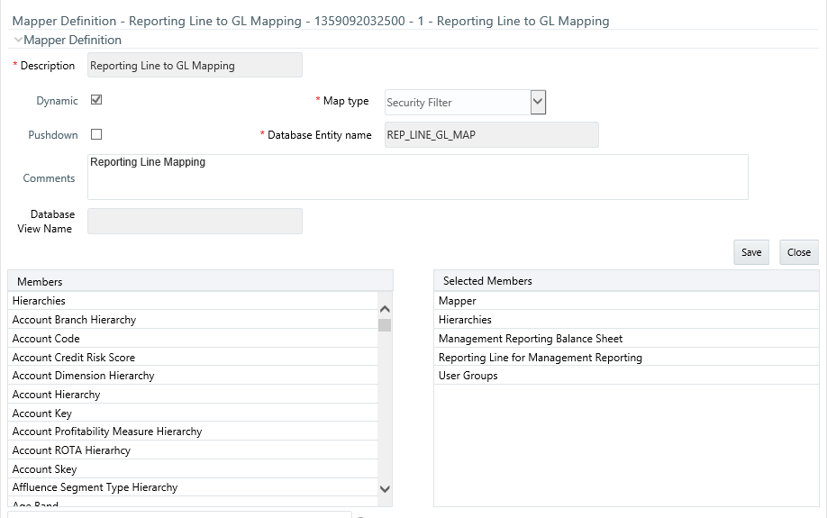
Similarly, a Mapper object provides the necessary reference to one or more hierarchies, when dimension/hierarchy data is needed to define conditional logic. In the example below, this map refers to a hierarchy created on the Organization Unit dimension.

Figure 5:   Mapper Definition- Reporting Line to GL Mapping

1.       To do the map maintenance, from the LHS menu, select Common Object Maintenance, select Unified Analytical Metadata, and then select Map Maintenance.

2.      Select the Add icon to create a new Map.

3.      On the left-hand side, select one or more hierarchies that were enabled in the initial step.

4.     Fill in the required information, for example, Name, Effective Dates, and Entity Name.

5.      Click Save.

6.     From the Map Maintenance summary page, select the Map, and then select the Mapper Maintenance icon.

Here, you will see the hierarchy and all parent/child relationships.

The range of product attributes supported for conditional assumptions and available for use within Data Filters is determined by columns that are part of the “Portfolio” definition. The “Portfolio” table class is seeded with the installation and can be extended to include user-defined columns.

For more information on adding user-defined columns to the Portfolio table class, see Chapter 2 - Object Management in Oracle Financial Services Data Model Utilities Guide.

When using mappers, Conditional Assumptions can be attached to any level of the hierarchy, allowing assumptions to be inherited from parent nodes by child nodes.

For example, you can use the Org Unit column to drive the assignment of Transfer Pricing Methods for all members of a particular Organization. You can create one Conditional Assumption to convey the entire Transfer Pricing Methodology logic and attach it to the top-level node of the Org Unit hierarchy. All nodes below the top-level node will inherit the same Transfer Pricing assumption.

The logic included in a Conditional Assumption determines the specific Transfer Pricing method, Prepayment assumption, or Adjustment Rule that the system will assign to each instrument record at run time.

The Conditional Assumption screen allows users to select explicit conditions (from Data Filters and/or Maps) and apply methods and rule selections to each condition directly. The Filter Conditions are processed by the engine in the order that they appear on the screen. As soon as a condition is satisfied, the related assumption is applied. The following screen shot displays a representative Conditional Assumption using a Data Filter:

Figure 6:   Conditional Assumptions

Conditional Assumptions can be applied only to detailed account records (data stored in the Instrument Tables). Instrument tables must have the TP - Cash Flow, Table Classification Code (200) in or order to use Conditional Assumptions.

Define Prepayment Rules

One of the major business risks faced by financial institutions engaged in the business of lending is prepayment risk. Prepayment risk is the possibility that borrowers might choose to repay part or all of their loan obligations before the scheduled due dates. Prepayments can be made by either accelerating principal payments or refinancing.

Prepayments cause the actual cash flows from a loan to a financial institution to be different from the cash flow schedule drawn at the time of loan origination. This difference between the actual and expected cash flows undermines the accuracy of transfer prices generated using cash flow based transfer pricing methods. Consequently, a financial institution needs to predict the prepayment behavior of instruments so that the associated prepayment risk is taken into account while generating transfer rates. Oracle Funds Transfer Pricing allows you to do this through the Prepayment Rule.

A Prepayment Rule contains methodologies to model the prepayment behavior of various amortizing instruments and quantify the associated prepayment risk. For more information, see Defining Transfer Pricing Methodologies.

Prepayment methodologies are associated with the product-currency combinations within the Prepayment rule. or more information, see Prepayment Rules.

Oracle Funds Transfer Pricing allows you to make use of the node level and conditional assumption while defining prepayment methodologies for your products. or more information, see Associating Node Level and Conditional Assumptions with Prepayment Rules.

Prepayment Methodologies and Rules

You can use any of the following four methods in a Prepayment rule to model the prepayment behavior of instruments:

·        Constant Prepayment Method

·        Prepayment Model Method

·        PSA Method

·        Arctangent Calculation Method

Constant Prepayment Method

The Constant Prepayment method calculates the prepayment amount as a flat percentage of the current balance.

You can create your origination date ranges and assign a particular prepayment rate to all the instruments with origination dates within a particular origination date range.

Prepayment Model Method

The Prepayment Model method allows you to define more complex prepayment assumptions compared to the other prepayment methods. Under this method, prepayment assumptions are assigned using a custom Prepayment model.

You can build a Prepayment model using a combination of up to three prepayment drivers and define prepayment rates for various values of these drivers. Each driver maps to an attribute of the underlying transaction (age/term or rate ) so that the cash flow engine can apply a different prepayment rate based on the specific characteristics of the record.

A typical Prepayment model structure includes the following:

·        Prepayment Drivers: You can build a Prepayment model using one to three prepayment drivers. A driver influences the prepayment behavior of an instrument and is either an instrument char­acteristic or a measure of interest rates.

·        Prepayment Driver Nodes: You can specify one or more node values for each of the prepay­ment drivers that you select.

·        Interpolation or Range method: Interpolation or Range methods are used to calculate prepay­ment rates for the prepayment driver values that do not fall on the defined prepayment driver nodes.

Types of Prepayment Drivers

Prepayment drivers are designed to allow the calculation of prepayment rates at run time depending on the specific characteristics of the instruments for which cash flows are being generated. Although nine prepayment drivers are available, a particular prepayment model can contain only up to three prepayment drivers.

Prepayment drivers can be divided into the following two categories:

·        Age/Term Drivers: The Age/Term drivers define term and repricing parameters in a Prepay­ment model. All such prepayment drivers are input in units of months. These drivers include:

§        Original Term: You can vary your prepayment assumptions based on the contractual term of the instrument. For example, you could model faster prepayment speeds for long-term loans, such as a 10-year loan, than for short-term loans, such as a 5-year loan. You would then select the Original Term prepayment driver and specify two node values: 60 months and 120 months.

§        Repricing Frequency: You can vary your prepayment assumptions based on the repricing nature of the instrument being analyzed. Again, you could specify different prepayment speeds for different repricing frequencies and the system would decide which one to apply at run time on a record by record basis.

§        Remaining Term: You can specify prepayment speeds based on the remaining term to maturity. For example, loans with few months to go until maturity tend to experience faster prepayments than loans with longer remaining terms.

§        Expired Term: This is similar to the previous driver but instead of looking at the term to maturity, you base your assumptions on the elapsed time. Prepayments show some aging effects such as the loans originated recently experiencing more prepayments than older ones.

§        Term to Repricing: You can also define prepayment speeds based on the number of months until the next repricing of the instrument.

·        Interest Rate Drivers: The Interest Rate drivers allow the forecasted interest rates to drive pre­payment behavior to establish the rate-sensitive prepayment runoff. Interest Rate Drivers include:

§        Coupon Rate: You can base your prepayment assumptions on the current gross rate on the instrument.

§        Market Rate: This driver allows you to specify prepayment speeds based on the market rate prevalent at the time the cash flows occur. This way, you can incorporate your future expec­tations on the levels of interest rates in the prepayment rate estimation. For example, you can increase prepayment speeds during periods of decreasing rates and decrease prepay­ments when the rates go up.

§        Rate Difference: You can base your prepayments on the spread between the current gross rate and the market rate.

§        Rate Ratio: You can also base your prepayments on the ratio of current gross rate to market rate.

The following diagram illustrates a three-driver prepayment model:

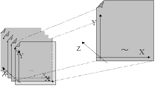
The ~ signifies a point on the X-Y-Z plane. In this example, it is on the second node of the Z-plane. The Z -plane behaves like layers.

Oracle Funds Transfer Pricing allows you to build prepayment models using the Prepayment Model rule. The Prepayment Model rule can then be referenced by a Prepayment Rule.

PSA Method

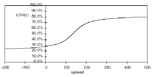
The PSA Prepayment method (Public Securities Association Standard Prepayment Model) is a standardized prepayment model that is built on a single dimension, remaining term. The PSA curve is a schedule of prepayments which assumes that prepayments will occur at a rate of 0.2 percent CPR in the first month and will increase an additional 0.2 percent CPR each month until the 30th month and will prepay at a rate of 6 percent CPR thereafter ("100 percent PSA"). PSA prepayment speeds are expressed as a multiple of this base scenario. For example, 200 percent PSA assumes annual prepayment rates will be twice as fast in each of these periods -- 0.4 percent in the first month, 0.8 percent in the second month, reaching 12 percent in month 30 and remaining at 12 percent after that. A zero percent PSA assumes no prepayments.

You can create your origination date ranges and assign a particular PSA speed to all the instruments with origination dates within a particular origination date range.

Arctangent Calculation Method

The Arctangent Calculation method uses the Arctangent mathematical function to describe the relationship between prepayment rates and spreads (coupon rate less market rate).

User defined coefficients adjust this function to generate differently shaped curves. Specifically:

CPRt = k1 - (k2 * ATAN(k3 * (-Ct/Mt + k4)))

where CPRt = annual prepayment rate in period t

Ct = coupon in period t

Mt = market rate in period t

k1 - k4 = user defined coefficients

A graphical example of the Arctangent prepayment function is shown below, using the following coefficients:

k1 = 0.3

k2 = 0.2

k3 = 10.0

k4 = 1.2

Each coefficient affects the prepayment curve in a different manner.

The following diagram shows the impact of K1 on the prepayment curve. K1 defines the midpoint of the prepayment curve, affecting the absolute level of prepayments. Adjusting the value creates a parallel shift of the curve up or down.

The following diagram shows the impact of K2 on the prepayment curve. K2 impacts the slope of the curve, defining the change in prepayments given a change in market rates. A larger value implies greater overall customer reaction to changes in market rates.

The following diagram shows the impact of K3 on the prepayment curve. K3 impacts the amount of torque in the prepayment curve. A larger K3 increases the amount of acceleration, implying that customers react more sharply when spreads reach the hurdle rate.

The following diagram shows the impact of K4 on the prepayment curve. K4 defines the hurdle spread: the spread at which prepayments start to accelerate. When the spread ratio = k4, prepayments = k1.

Associating Node Level and Conditional Assumptions with Prepayment Rules

You can define prepayment methodologies at any level of the product hierarchy. Children of a hierarchical node automatically inherit the assumptions defined at the parent level. Methodologies directly defined for child nodes take precedence over those defined at the parent level. For more information, see Defining Transfer Pricing Methodologies Using Node Level Assumptions.

You can also use the conditional logic of Conditional Assumptions to define prepayment methodologies based on particular characteristics of financial instruments. For more information, see Associating Conditional Assumptions with Assumption Rules.

Define Adjustment Rules

Adjustment Rules allow users to define Transfer Pricing Add-on rates that are assigned incrementally to the base FTP rate to account for a variety of miscellaneous risks such as Liquidity risk or Basis risk or to supplement strategic decision making through the use of Pricing Incentives, Breakage Charges or other types of rate adjustments.

Within both the Standard and Stochastic Transfer Pricing Processes, users can select an appropriate Adjustment rule to calculate add-on rates or breakage charges.

Add-on rates can be a fixed rate, a fixed amount, or a formula based rate. Breakage Charges can be a fixed percentage, a fixed amount or can be calculated on an Economic Loss basis. The adjustments are calculated and output separately from the base funds transfer pricing rate, so they can be easily identified and reported. Also, Adjustments allow you to apply event-based logic through the use of conditional assumptions that are applied or varied only if a specific condition is satisfied.

Adjustment Methods and Rules

You can use any of the following methods in an Adjustment rule when the selected Adjustment Type is Liquidity Premium, Basis Risk Cost, Pricing Incentive, or Other Adjustment:

·        Fixed-Rate

·        Fixed Amount

·        Formula Based Rate

·        Use TP Method from selected TP Rule

Alternatively, you can use any of the following methods in an Adjustment rule when the selected Adjustment Type is Breakage Charge:

·        Economic Loss

·        Fixed Amount

·        Fixed Percentage

Adjustment - Fixed Rate

Figure 7:   Adjustment Rule Details

The Fixed Amount Adjustment method allows the user to associate an amount with specific terms or term ranges. Reference term selections include

·        Repricing Frequency: The fixed amount is matched to the specified reprice frequency of the instrument. If the instrument is fixed rate and, therefore, does not have a reprice frequency, the fixed amount lookup happens based on the original term of the instrument.

·        Original Term: The calculation assigns the fixed amount based on the original term on the instrument.

·        Remaining Term: The calculation assigns the fixed amount based on the remaining term of the instrument.

The remaining term value represents the remaining term of the contract and is expressed in days.

Remaining Term = Maturity Date – As of Date

·        Duration (read from the TP_DURATION column): The calculation assigns the fixed amount based on the Duration of the instrument, specified in the TP_DURATION column.

·        Average Life (read from the TP_AVERAGE_LIFE column): The calculation assigns the fixed amount based on the Average Life of the instrument, specified in the TP_AVG_LIFE column.

You can create your reference term ranges and assign a particular adjustment amount to all instruments with a reference term falling within the specified range.

Adjustment - Fixed Amount

Figure 8:   Adjustment Rule Details

The Fixed Amount Adjustment method allows the user to associate an amount with specific terms or term ranges. Reference term selections include:

·        Repricing Frequency: The calculation retrieves the rate for the term point equaling the reprice frequency of the instrument. If the instrument is fixed rate and, therefore, does not have a reprice frequency, the calculation retrieves the rate associated with the term point equaling the original term on the instrument.

·        Original Term: The calculation retrieves the rate for the term point equaling the original term on the instrument.

·        Remaining Term: The calculation retrieves the rate for the term point corresponding to the remaining term of the instrument. The remaining term value represents the remaining term of the contract and is expressed in days. Remaining Term = Maturity Date – As of Date

·        Duration (read from the TP_DURATION column): The calculation retrieves the rate for the term point corresponding to the Duration of the instrument, specified in the TP_DURATION col­umn.

·        Average Life (read from the TP_AVERAGE_LIFE column): The calculation retrieves the rate for the term point corresponding to the Average Life of the instrument, specified in the TP_AVG_LIFE column.

You can create your reference term ranges and assign a particular adjustment amount to all instruments with a reference term falling within the specified range.

Adjustment - Formula Based Rate

Figure 9:   Adjustment Rule Details - Formula Based Rate

The Formula Based Rate Adjustment method allows the user to determine the add-on rate based on a lookup from the selected yield curve, plus a spread amount, and then the resulting rate can be associated with specific terms or term ranges. Reference term selections include:

·        Repricing Frequency: The calculation retrieves the rate for the term point equaling the reprice frequency of the instrument. If the instrument is fixed rate and, therefore, does not have a reprice frequency, the calculation retrieves the rate associated with the term point equaling the original term on the instrument.

·        Original Term: The calculation retrieves the rate for the term point equaling the original term on the instrument.

·        Remaining Term: The calculation retrieves the rate for the term point corresponding to the remaining term of the instrument. The remaining term value represents the remaining term of the contract and is expressed in days.

Remaining Term = Maturity Date – As of Date

·        Duration (read from the TP_DURATION column): The calculation retrieves the rate for the term point corresponding to the Duration of the instrument, specified in the TP_DURATION col­umn.

·        Average Life (read from the TP_AVERAGE_LIFE column): The calculation retrieves the rate for the term point corresponding to the Average Life of the instrument, specified in the TP_AVG_LIFE column.

You can create your own reference term ranges and assign a particular formula based adjustment rate to all instruments with a reference term falling within the specified range.

With this method, you also specify the Interest Rate Code and define an Assignment Date for the Rate Lookup. The Interest Rate Code can be any IRC defined within Rate Management, but will commonly be a Hybrid IRC defined as a Spread Curve (for example, Curve A – Curve B).

Assignment Date selections include:

·        As of Date

·        Last Repricing Date

·        Origination Date

·        TP Effective Date

·        Adjustment Effective Date

·        Commitment Start Date

Each term range additionally allows users to input a Rate Cap and a Rate Floor. These boundaries will only apply to the 'Formula Based method' and 'Use TP Method from TP Rule' based adjustments. These are optional inputs. This input will limit the Max or Min rate regardless of the rate passed by the Formula/TP Rule. Sometimes, there may be major external events that cause a short term spike in rates and certain accounts may be negatively impacted as a result. Applying a rate cap (or floor) will allow business users to limit these spikes.

The formula definition is comprised of the following components

Figure 10:   Adjustment Rate Details

·        Term Point: Allows you to associate a specific term point from the IRC to each Term Range.

·        Coefficient: Allows you to define a multiplier that is applied to the selected rate.

·        Rate Spread: Allows you to define an incremental rate spread to be included on top of the IRC rate.

The resulting formula for the adjustment rate is: (Term Point Rate * Coefficient) + Spread

For example:

Figure 11:   Formula Rate Parameters

Adjustment - Use TP Method from Selected TP Rule

The "Use TP Method from Selected TP Rule" selection allows the user to calculate the add-on rate based on any TP method available in the selected Transfer Pricing Rule.

Figure 12:   Adjustment Rule Details - TP Method

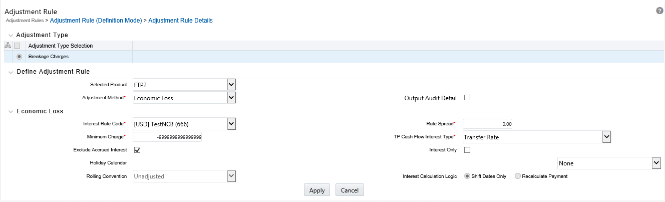
Users have the option to attach any Transfer Pricing Rule on the Adjustment Rule summary page, separately for each type of add-on rate. The TP Methods mapped to product hierarchy members in the TP Rule will be read during the adjustment rate calculation process and will be applied during the calculation of the Adjustment Rate(s). Outputs will be written to the respective Adjustment Rate column, for example, Basis Risk Cost Rate, Liquidity Premium Rate, Pricing Incentive Rate, or Other Adjustment Rate.

·        Term:

§        Standard Term: Adjustment would be calculated as per the repricing period for adjustable rate instruments and use original term (maturity date - origination date) for fixed rate instru­ments.

§        Original Term: Adjustments would be calculated as per the original term like a fixed rate instrument.

Figure 13:   Adjustment Rule Details

Breakage Charges

A breakage charge represents the cost of breaking a contractual obligation. In Bank Finance this typically means the early prepayment of a loan by a customer or the early withdrawal of deposit funds by a customer. “Early” in this sense means before the contractual maturity date.

The gain or loss to the Bank from such early prepayments and withdrawals is the opportunity cost of not being able to replace the spread earned on the asset or deposit being lost. For example, the early withdrawal of funds from a 2-year term deposit exposes the bank to the risk of replacing that funding in a higher rate environment and thereby reducing the net interest margin earned before the withdrawal. With matched-term transfer pricing, this risk is split between the Line Unit and Treasury. The Line Unit holds the risk of deteriorating credit spread, but Treasury holds the funding risk (the risk that the funding spread between the Bank's assets and liabilities will narrow).

There are three Breakage Charge methods available including:

·        Economic Loss

·        Fixed Amount

·        Fixed Percentage

Breakage Charge – Economic Loss

Figure 14:   Adjustment Rule Details - Adjustment Method as Economic Loss

The Economic Loss breakage charge method sets out to compute the cost to the organization (economic loss) incurred for terminating the funding liability (also known as the shadow liability). The calculation assumes the funding liability has the exact attributes of the funded/terminated instrument. The rate of the funding liability is equal to the Transfer Rate. Economic Loss is computed as follows:

For Assets:

Economic Loss =BV - MV

For Liabilities:

Economic Loss = MV– BV

Where:

MV: Market Value of the funding Liability

BV: Book Value of the broken instrument

The following is a simplified example of the Economic Loss calculation for a standard Term Deposit:

Book Value: $1,000.00

Original Term: 24 Months

Break after: 12 Months

Original TP Rate: 2.40% (based on straight term method)         

Breakage Charge – Fixed Amount

Figure 15:   Adjustment Rule Details - Adjustment Method as Fixed Amount

The Fixed Amount method allows users to directly input the amount of the breakage charge. This method would typically be used in cases where the cash flows and Economic Loss method are not appropriate for determining the breakage cost.

The only input required for this method is the breakage charge amount.

Breakage Charge - Fixed Percentage

Figure 16:   Adjustment Rule Details - Adjustment Method as Fixed Percentage

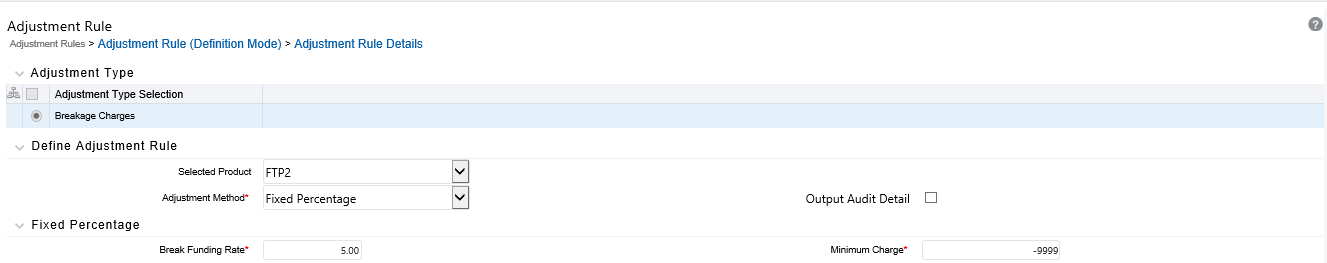
An alternative to the Fixed Amount method, the Fixed Percentage approach allows you to input a percentage that is multiplied by the breakage amount to determine the breakage charge.

Calculation:

Breakage Charge = Break Amount x (Charge % / 100)

If the resulting amount is greater than the specified minimum charge, the calculated amount is output. Otherwise, the minimum charge will be output.

Pre-requisites for calculating Breakage Charges

1.       Break event records should be populated in the FSI_D_BREAK_FUNDING_CHARGES table. This can be done directly through a manual data loading process or can be automated using an FTP Break Identification Process. (see Break Identification Process, on page 537)

2.      An Adjustment Rule should be defined with Breakage Charge assumptions created for all of the relevant Product / Currency combinations (see Adjustment Rules, on page 471)

3.      A Standard TP Process should be defined with the following: (see Transfer Pricing Process)

§        The Break Funding Charges table selected on the Product Selection block

§        Adjustments must be selected on the Calculation Elements block

§        An Adjustment Rule containing the required Breakage Charge assumptions must be selected

Associating Node Level and Conditional Assumptions with Adjustment Rules

You can define adjustment methods at any level of the product hierarchy. Children of a hierarchical node automatically inherit the assumptions defined at the parent level. Methodologies directly defined for child nodes take precedence over those defined at the parent level. For more information, see Defining Transfer Pricing Methodologies Using Node Level Assumptions.

You can also use the conditional logic of Conditional Assumptions to define Adjustment methods based on the particular characteristics of your financial instruments. For more information, see Associating Node Level and Conditional Assumptions with Prepayment Rules.

Define Alternate Rate Output Mapping Rules

Within the Standard Transfer Pricing Process, users can select an appropriate Alternate Rate Output Mapping rule to output transfer pricing results to the seeded or user-defined alternate columns instead of the standard default column.

The Alternate Rate Output Mapping rule lets you select the alternate columns to output transfer rate, option cost, and adjustment calculation results for each instrument record for a transfer pricing process run. This functionality allows you to output more than one transfer rate, option cost, or adjustment calculation result for each instrument record through multiple transfer pricing process runs.

For example, you may run Oracle Funds Transfer Pricing once without selecting an Alternate Rate Output Mapping rule and thus use the original default output columns, such as TRANSFER_RATE and MATCHED_SPREAD_C, to store transfer pricing results. You may then run the application a second or third time using an Alternate Rate Output Mapping rule in different Transfer Pricing Processes, which run against the same instrument records. The result would be two or three transfer rates, option costs, or adjustment calculation results populated into distinct columns for each instrument record in the specified Instrument tables.

Define and Execute a Transfer Pricing Process

Defining and executing a Transfer Pricing Process is one of the mandatory steps in Oracle Funds Transfer Pricing. The Transfer Pricing Process allows you to:

·        Select transfer pricing, prepayment, and adjustment assumptions, respectively contained in the associated Transfer Pricing, Prepayment, and Adjustment rules, within the Transfer Pricing Pro­cess.

·        Determine the data that you want to process in a particular run.

·        Define the calculation elements used in transfer rate, option cost, economic value, and adjust­ment calculations, also, to migrate transfer pricing results to the Management Ledger table.

·        Choose the calculation mode for generating transfer pricing results, such as the Remaining Term or Standard.

·        Select which calculations, such as Transfer Rates, TP Rate Adjustments, or Option Costs to per­form.

·        Optionally select an Alternate Rate Output Mapping Rule. Alternate Rate Output Mapping rules can be used when you want to direct the FTP output to non- standard columns.

Once a Transfer Pricing Process has been created, a user may select RUN from the summary page to execute it.

When a Transfer Pricing Process rule is executed, detailed records are processed and individual records are updated with the results of the transfer pricing process. These results are based on the calculation elements selected.

The following table displays the Instrument table fields that may be updated as a result of transfer pricing processing when you select Account tables as the data source.

Instrument Table Fields Updated by Transfer Pricing Processing:

Additionally, you may choose the Ledger table as the data source for the transfer pricing of certain products. If the Ledger table data source is selected, the following rows are created for each product:

·        Financial Element 170, Average Transfer Rate

·        Financial Element 450, Charge/Credit

·        Financial Element 172, Average Remaining Term Transfer Rate

·        Financial Element 452, Charge/Credit Remaining Term

TP_EFFECTIVE_DATE and ADJUSTMENT_EFFECTIVE_DATE are used by the FTP Standard Process as an override date for determining the historical rate from the specified interest rate curve (IRC). TP_EFFECTIVE_DATE and ADJUSTMENT_EFFECTIVE_DATE are typically used in cases where the customer rate on the instrument record is set before the origination date and users wish to align the TP Rate lookup with the date that the customer rate was set.

The FTP process normally uses the ORIGINATION_DATE for fixed-rate instruments or LAST_REPRICE_DATE for adjustable-rate instruments to determine historical rate effective date for the transfer rate or Adjustment Rate lookup. This input allows users to specify an alternate effective date.

If applicable, set the TP_EFFECTIVE_DATE = ISSUE_DATE or the date on which the customer rate was set.

·        TP_EFFECTIVE_DATE should be NULL if not applicable. Do not default TP_EFFECTIVE_DATE (for example, 01-JAN-1900) to a valid date as the TP Engine will reference any valid date.

·        TP_EFFECTIVE_DATE <> ORIGINATION_DATE

·        TP_EFFECTIVE_DATE <> LAST_REPRICE_DATE

Transfer Pricing Process and the Propagation Pattern

Transfer Pricing theory suggests that a Transfer Rate on a fixed-rate instrument should apply throughout its entire life (for Fixed Rate Instruments) or Repricing Term (for Adjustable Rate Instruments). We apply this theory to Transfer Rate propagation.

The Propagation Patterns allow you to pull forward (propagate) the Transfer Rate and Matched Spread on any applicable instrument record from a prior period of history. Propagation methodologies are defined at the application level and apply to all TP process rules.

When Propagation is run in a single process, together with Transfer Pricing rate calculations, the TP Engine will first propagate rates and then will calculate rates for the remaining un-priced records.

The Propagation process will generally refer to details on the individual instrument records to determine if Transfer Rates are eligible for propagation.

For example,

·        If an instrument is a fixed rate, then propagate.

·        If an instrument is adjustable, and a repricing has not occurred between the prior period and current period, then propagate.

In addition to the above general logic, if Transfer Rate calculation is also selected in the same TP Process, then an additional test to confirm whether the TP Method for the applicable products is a “Bulk update” TP method then additionally, propagation will not happen for related instrument records.

The test to determine if a TP method is a bulk method is as follows:

Spread from Interest Rate Code with mid-period repricing not selected

Moving Average

Spread from Interest Rate Code or Redemption Curve with mid-period repricing not selected and Origination Date = As of Date

The Standard Transfer Pricing Process allows you to propagate Transfer Rates and Adjustment Rates, and the Stochastic Transfer Pricing Process allows you to propagate Options Costs and Adjustment Rates. Depending upon your requirements, you can choose to propagate prior period results on the Transfer Pricing Calculation Selection block.

The main goal of using propagation is to improve performance. Since Propagation uses a bulk processing approach, it provides a significant performance improvement over processing instruments with a row-by-row approach. Although precise performance numbers may vary depending on the hardware and database configuration, processing a set of instrument records using propagation is significantly faster than doing it on the same set of records on a row-by-row basis.

Transfer Pricing Process and Audit Options

Transfer Pricing Processes provide you with three audit options: Detailed Cash Flow, Forward Rates, and 1 Month Rates. While Detailed Cash Flow audit option applies to both Standard and Stochastic TP Processes, the Forward Rates and 1 Month Rates audit options are applicable only to Stochastic TP processing.

By selecting the Detail Cash Flow option in the Transfer Pricing Process Audit block, you can audit daily cash flow results generated by the Oracle Funds Transfer Pricing application. Selecting this option writes out all cash flow and repricing events that occur for processed records. The number of records written is determined by the user based on the value input for the Number of Records.

The relevant financial elements for each instrument record and the cash flow results are stored in the FSI_O_PROCESS_CASH_FLOWS table.

After processing cash flows from Transfer Pricing, do the following to view the audit results:

·        Determine the value of the ID Numbers for the instruments that you want to process.

·        View data by:

§        Querying the FSI_O_PROCESS_CASH_FLOWS table with Oracle SQL Developer, SQL Plus, Toad, or an equivalent SQL query tool.

SQL Query Results

The results of running a SQL query can be exported to an Excel file for validation.

Financial Elements

The FINANCIAL_ELEMENT_ID column lists the financial elements written for each payment and repricing event processed by the cash flow engine. An initial set of data is also written, recording the balance and rate as of the last payment date.

The following table describes the financial elements that can be present in a base set of financial elements written during a cash flow audit process:

Cash Flow Codes

The Cash Flow Code column lists a code for each row that describes the event modeled by the cash flow engine.

The following table describes the different cash flow codes:

Data Verification

You can export results from your SQL query into Excel format and use Excel to validate the results. If the cash flows do not behave as expected, examine instrument table data or your assumptions. For more information on Cash Flow Calculations, see the Oracle Financial Services Cash Flow Engine Reference Guide.

Transfer Pricing Process Rule and Calculation Modes

You can choose to transfer price your product portfolio either in the Standard or in Remaining Term calculation mode.

The Standard calculation mode allows you to calculate transfer rates for instrument records based on the Origination date or Last Repricing Date of the instruments. It can also be used to calculate Option Costs based on the Origination Date.

The Remaining Term calculation mode allows you to calculate transfer rates and option costs for instrument records based on the remaining term of the instrument from the calendar period end date of the data, rather than the Origination Date or Last Repricing Date of the instruments.

The Remaining Term calculation mode treats your portfolio as if you acquired it on the As of Date of your data and thereby allows you to measure current rate risk spread. Once you know the current rate risk spread, you can segregate your total rate risk spread into that accruing from taking current rate risk and that accruing from taking embedded rate risk:

Embedded Rate Risk Spread = Total Rate Risk Spread - Current Rate Risk Spread

It is important to segregate total rate risk into embedded and current rate risks for the following reasons:

·        The current rate risk can be actively managed through an effective Asset/Liability Management process.

·        Embedded rate risk is a result of rate bets taken in the past. However, it is important to measure and monitor this risk. When you are aware of your embedded rate risk you will neither be lulled into a false sense of security or take drastic actions in response to profit or losses caused by the embedded rate risk.

Transfer Pricing Process and Migration Options

The purpose of the Ledger Migration process is to generate dollar charges or credits for funds provided or used for a combination of dimensions. The information necessary to generate these charges or credits (through transfer rates, adjustments, and option cost processing) originates from the Instrument Tables and the results are inserted into the Management Ledger table and are available for use in the calculation of profitability and risk measures.

Within the Transfer Pricing Process definition screen, on the "Migration" block, users can select from 2 options for the charge/credit method:

·        Account Level: The Account Level method will sum the charge/credit amounts computed at the individual instrument level (based on the instrument's current or average book balances) and will group the results by the set of selected dimensions and migrate the amounts, together with the weighted average transfer rates to the Management Ledger table.

·        Ledger Level: The Ledger Level method will compute the weighted average transfer rates from the instrument data and will migrate these values to the Management Ledger table. The migra­tion process will then multiply the weighted average transfer rates by the Ending or Average bal­ances on the Management Ledger Table to arrive at the TP charge or credit amounts.

The following Migration – Charge/Credit Methods are available:

With both methods, the following rows are created for each product (and combination of selected dimensions). An offset entry to the funding center (offset org unit) is also created.

When Transfer Rate is selected (based on Standard or Remaining Term option):

·        Financial Element 170, Average Transfer Rate

·        Financial Element 450, Charge/Credit

·        Financial Element 172, Average Remaining Term Transfer Rate

·        Financial Element 452, Charge/Credit Remaining Term

When Adjustments are selected (based on the population of noted adjustment type):

·        Financial Element 174, Average Liquidity Adjustment Rate

·        Financial Element 414, Liquidity Adjustment Charge/Credit

·        Financial Element 175, Average Basis Risk Cost Rate

·        Financial Element 415, Basis Risk Cost Charge/Credit

·        Financial Element 176, Average Pricing Incentive Rate

·        Financial Element 416, Pricing Incentive Charge/Credit

·        Financial Element 177, Average Other Adjustment Rate

·        Financial Element 417, Other Adjustment Charge/Credit

When Option Costs are selected: (based on Standard or Remaining Term option)

·        Financial Element 171, Average Historic Option Cost

·        Financial Element 451, Historic Option Cost Charge/Credit

·        Financial Element 173, Average Current Option Cost

·        Financial Element 453, Current Option Cost Charge/Credit

Oracle Funds Transfer Pricing provides great flexibility in the ledger migration process and the generation of corresponding charges and credits. Users can specify ledger migration for a combination of an extended list of dimensions, including organizational unit, product, channel, GL account, geography, or any other dimension that is part of the key dimension set.

You can choose to migrate the transfer rate, adjustment amounts, or the option costs, within the respective Standard or Stochastic Transfer Pricing Process.

Transfer Pricing Process and Calculating Economic Value

You can choose to calculate Economic Value as part of a Standard Transfer Pricing Process by selecting the Economic Value calculation element. This calculation option refers to the Economic Value assumptions defined within the Transfer Pricing rule and is also eligible for Alternate Rate Output mapping. Additionally, there are seeded output columns available corresponding to each of the seeded interest type elements.

All Transfer Rate types (Transfer Rate, Transfer Rate Alt, Remaining Term Transfer Rate, and Remaining Term Transfer Rate Alt) will be written to a single/shared column, Economic Value Transfer Rate (EV_TP_RATE). If it is necessary to store more than one of these EV outputs, Alternate Rate Output mapping can be used. Each type of Adjustment Rate is mapped to its corresponding EV column. For example:

·        Economic Value Liquidity Premium Rate - EV_LIQ_PREM_RATE

·        Economic Value Basis Risk Rate - EV_BASIS_RISK_RATE

·        Economic Value Pricing Incentive Rate - EV_PRIC_INC_RATE

·        Economic Value Other Adjustment Rate - EV_OTH_ADJ_RATE

·        Economic Value Other Adjustment Alternate Output - EV_OTH_ADJ_RATE_ALT

Also, the All-in TP Rate is mapped to a corresponding EV column.

Economic Value All in Transfer Rate - EV_ALLIN_TP_RATE

The output format for the Economic Value calculation (inputs defined through the Transfer Pricing rule) is as follows:

For Assets:

·        Economic Value = MV - BV

For Liabilities:

·        Economic Value = BV– MV

where

BV = Book Value = CUR_BOOK_BAL

MV = Market Value = Net Present Value of Principal (FE210) and Interest (FE430) Cash Flows

In addition to the above calculation logic, users can specify the following two parameters:

·        Interest Only: If this option is selected, the Net Present Value calculation considers only the Interest Cash Flows (FE430). In this case, the output format is as follows:

Economic Value = MV

·        Exclude Accrued Interest: If this option is selected, the first interest cash flow will be computed from the As of Date to the Next Payment Date. The resulting market value will reflect the clean price.

In the case of forward starting instruments, that is, instruments that are not yet on the balance sheet, that is, ORIGINATION_DATE > AS_OF_DATE, The logic for computing Economic Value is as follows:

Economic Value =MV

Stochastic Transfer Pricing Process and Option Cost Parameters

In addition to transfer rates (created by a Standard TP Process), the Stochastic Transfer Pricing Process allows you to calculate the cost of options that are associated with your instruments. If you want to calculate option costs, you need to define the parameters used in option costing within the Stochastic Transfer Pricing Process.

The purpose of option cost calculations is to quantify the cost of optionality, in terms of a spread over the transfer rate, for a single instrument. The cash flows of an instrument with an optionality feature change under different interest rate environments and thus should be priced accordingly.

For example, many mortgages can be prepaid by the borrower at any time without penalty. In effect, the lender has granted the borrower an option to buy back the mortgage at par, even if interest rates have fallen in value. Thus, this option has a cost to the lender and should be priced accordingly.

In another case, an adjustable-rate loan may be issued with rate caps (or floors) which limit its maximum (or minimum) periodic cash flows. These caps and floors constitute options.

Such flexibility given to the borrower raises the bank's cost of funding the loan and will affect the underlying profit. The calculated cost of these options may be used in conjunction with the transfer rate to analyze profitability.

Oracle Funds Transfer Pricing uses the Monte Carlo technique to calculate the option cost. Oracle Funds Transfer Pricing calculates and outputs two spreads and the related option cost (rate) which is the difference between these two spreads. The two spreads are:

·        Static spread (HISTORIC_STATIC_SPREAD)

·        Option-adjusted spread (HISTORIC_OAS)

The option cost is derived as follows:

·        Option cost (rate) = OAS – Static Spread

The Option Cost calculation process will also compute the charge/credit amount using the Option Cost (rate), Average Balance, and Accrual Factor and will write the result to the following column:

·        CHARGE_CREDIT_OCOST

The static spread is equal to margin and the OAS to the risk-adjusted margin of an instrument. Therefore, the option cost quantifies the loss or gain due to risk. For more information on Transfer Pricing Option Cost, see the Oracle Financial Services Cash Flow Engine Reference Guide.

Stochastic Transfer Pricing Process and Stochastic Rate Indexing Rules

The Stochastic Rate Indexing rule is one of the assumption rules that you need to select within a Stochastic Transfer Pricing Process to calculate option costs.

The purpose of the Stochastic Rate Indexing Rule is to establish relationships between a risk-free Interest Rate Code (IRCs) and other interest rate codes or Indexes. The Stochastic Rate Indexing rule allows you to select the valuation curve that the system uses during stochastic processing. The Rate Index rule provides full support for multi-currency processing by allowing you to select one valuation curve per currency supported in your system.

During stochastic FTP processing, the system generates future interest rates for the valuation curve you selected, which are then used to derive the future interest rates for any Index associated with that valuation curve based on the relationship you define. The rates thus forecasted for the IRCs or Indexes depend on the risk-free curve used for the valuation of instruments associated with the derived IRCs or Indexes. As the risk-free rates change, the non-risk-free interest rates change accordingly.

Define and Execute a Break Identification Process

Break Identification processing should be run if automatic break detection is the preferred approach to populating the break events table (FSI_D_BREAK_FUNDING_CHARGES). Users also have the option to populate this table manually during data loading or use a hybrid approach. The Break Funding Charges table is the source table for calculating breakage charges.

To complete the breakage charge calculation process, after populating breakage data, the Break Funding Charges table should be selected in a Transfer Pricing Process as the source table and the calculate Adjustments option should be selected under Calculation Selection. Finally, an appropriate Adjustment Rule (containing Breakage Charge assumptions), should be selected in the TP Process to apply the desired Breakage Charge calculation method.

The Break Identification Process supports 4 Break Types:

·        Full Break (type 1)

·        Partial Break (type 2)

·        Change in Attributes (type 3)

·        Partial Break + Change in Attributes(type 5)

Assumptions

1.       It is assumed that instruments that are fully repaid or terminated will not be available in the instrument table for the current period. If users choose to include fully re-paid instruments, in the current data, these records should have a current balance of zero and account open flag = No.

2.      Records will be identified and compared uniquely based on the ID Numbers. It is assumed that the ID Numbers will not be duplicated for a given period within an instrument table.

3.      Both current and prior period data exist in the same instrument table. The current period refers to As of Date specified in FTP Application Preferences. A prior period is calculated based on assumptions given in the Break Identification Process.

4.     When the Nearest Prior Date option is selected in the Break Identification Process for determining the prior period as of date, it is assumed that the process has been previously executed and an entry exists in the Process Run History table.

The following data flow illustrates how Break Identification processing works in the context of the overall staging and instrument table design:

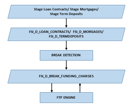
The following figure shows the overview of Break Identification process:

Full Breaks

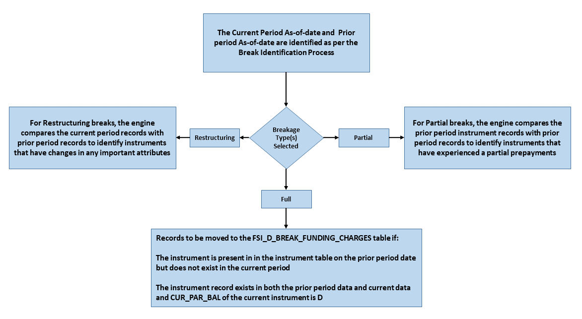
The following accounts are considered as full breaks, fully repaid or terminated:

·        The Instrument is present in the instrument table on the prior period date but does not exist in the current period and the maturity date of the prior period record is greater than the current period as of the date.

·        The Instrument record exists in both the prior period data and current data and CUR_PAR_BAL of the current instrument is 0 and the account open flag is NO.

For the above scenarios, the Break Identification Process populates the source and Break Funding Charges instrument tables with the following:

·        BREAKAGE_FLG = 2 (*Source record only) (External break will populate flag=1)

·        BREAKAGE_TYPE_CD = 1

·        BREAKAGE_AMOUNT = CUR_PAR_BAL (prior period)

Additionally, the FSI_D_BREAK_FUNDING_CHARGES table is populated as follows:

·        If Prior record NEXT_PAYMENT_DATE > Current AS_OF_DATE then:

§        CUR_PAR_BAL = Prior Period CUR_PAR_BAL

§        CUR_BOOK_BAL = Prior Period CUR_BOOK_BAL

·        If Prior record NEXT_PAYMENT_DATE <= Current AS_OF_DATE then:

§        CUR_PAR_BAL = AFTER_PAYMENT_BALANCE

§        CUR_BOOK_BAL = AFTER_PAYMENT_BALANCE

·        AS_OF_DATE = AS_OF_DATE defined in Application Preferences

·        BREAKAGE_AMOUNT = Prior Period CUR_PAR_BAL

·        BREAKAGE_TYPE_CD = 1

·        All additional fields are carried forward from the prior period record

For Full Breaks, Next Payment Date gets rolled forward till Maturity Date. Break record has AS_OF_DATE = NEXT_PAYMENT_DATE.

If NEXT_PAYMENT_DATE <= AS_OF_DATE, then Next Payment Date = Next Payment Date + Payment Frequency/Multiplier. This should not exceed the Maturity Date.

If NEXT_PAYMENT_DATE <= AS_OF_DATE for the current period, then Break Amount = AFTER_PAYMENT_BAL from the prior record. This is used when you do not want to pay a break charge against the current period's scheduled principal payment.

Partial Breaks

For partial breaks, the engine compares the prior period instrument records with current period records to identify instruments that have experienced a partial prepayment.

The Break Identification Process uses Identity Code to determine which record is current and which is prior. It is assumed the Prior record Identity Code will be < Current Period.

The following accounts are considered as partial breaks:

Case 1

 If the NEXT_PAYMENT_DATE on the prior period record is less than or equal to the AS_OF_DATE of the current period record, then:

·        To detect a partial break, compare the AFTER_PAYMENT_BALANCE of the prior period record with the CUR_PAR_BAL of the current period record. If the difference is more than the MINI­MUM_BREAK_AMOUNT then the instrument is classified as a Partial Break.

For the above scenario, the Break Identification Process populates the source and Break Funding Charges instrument tables with the following:

§        BREAKAGE_FLG = 2 (*Source - Current record only) (External break will populate flag=1)

§        BREAKAGE_TYPE_CD = 2

§        BREAKAGE_AMOUNT = AFTER_PAYMENT_BALANCE of prior record – CUR_PAR_BAL of the current record

Additionally, the FSI_D_BREAK_FUNDING_CHARGES table is populated as follows:

§        Both the prior period record and the current record are copied into the FSI_D_BREAK_FUND­ING_CHARGES table. The as of date for the prior record is changed to the current as of date.

§        The BREAKAGE_AMOUNT of the prior record =0

§        The BREAKAGE_AMOUNT of the current record = AFTER_PAYMENT_BALANCE of prior record – CUR_PAR_BAL of the current record

§        BREAKAGE_TYPE_CD = 2

§        Specific Fields updated on prior break funding record:

—     Next Payment Date: If Next Payment Date <= AS_OF_DATE then Next Payment Date +Payment Frequency/Multiplier

—     Last Payment Date: If Next Payment Date <= AS_OF_DATE then Next Payment Date

—     Next Reprice Date: If Next Reprice Date <= AS_OF_DATE then Next Reprice Date + Reprice Frequency/Multiplier

—     Last Reprice Date: If Next Reprice Date <= AS_OF_DATE then Next Reprice Date

—     Remaining Number of Payments: If Next Payment Date <= AS_OF_DATE then Remaining Number of Payments -1

§        All additional fields are carried forward from the prior period record

Case 2

If the NEXT_PAYMENT_DATE on the prior period record is greater than the as of date of the current period, then:

·        To detect a partial break, compare the CUR_PAR_BAL of the prior period record with the CUR_PAR_BAL of the current record. If the difference is more than the Minimum Break Amount, then the instrument is classified as a partial break.

For the above scenario, the Break Identification Process populates the source and Break Funding Charges instrument tables with the following:

§        BREAKAGE_FLG = 2 (*Source - Current record only)

§        BREAKAGE_TYPE_CD = 2

—     If both Partial and Change in Attributes are detected, then BREAKAGE_TYPE_CD = 5

§        BREAKAGE_AMOUNT = CUR_PAR_BAL of the prior period record – CUR_PAR_BAL of the current record

Additionally, the FSI_D_BREAK_FUNDING_CHARGES table is populated as follows:

§        Both the prior period record and the current record are copied into the FSI_D_BREAK_FUND­ING_CHARGES table. The as of date for the prior record is changed to the current as of date.

§        The BREAKAGE_AMOUNT of the prior record =0

§        The BREAKAGE_AMOUNT of the current record = CUR_PAR_BAL of prior record – CUR_PAR_BAL of current record

§        BREAKAGE_TYPE_CD = 2

§        RECORD_IND = -1 for Prior Record and 1 for Current Record

§        All additional fields are carried forward from the prior period record

Example - Partial Break:

·        Prior Record:

§        As-of-date = 30-SEP-2012

§        Next_reprice_Date = 01-OCT-2012

§        Last_reprice_date = 01-SEP-2012

§        REPRICE_FREQ = 1M

·        Current Record:

§        As-of-date = 01-OCT-2012

§        Next_reprice_Date = 01-NOV-2012

§        Last_reprice_date = 01-OCT-2012

§        REPRICE_FREQ = 1M

The break occurs on 01-OCT-2012 and break is detected on this date. This is also the Application Preferences As of Date given by the user.

Records moved to FSI_D_BREAK_FUNDING_CHARGES will be:

·        Prior Record:

§        Since next_reprice_Date (1-Oct-2012) <= active as of date (1-Oct-2012),

§        As_of_date = 01-OCT-2012

§        Next_reprice_date = 01-NOV-2012

§        Last_reprice_date = 01-OCT-2012

·        Current Record:

§        As_of_date = 01-OCT-2012

§        Next_reprice_date = 01-NOV-2012

§        Last_reprice_date = 01-OCT-2012

§        The engine can only process the modified record in FSI_D_BREAK_FUNDING_CHARGES when Last_reprice_date <= as_of_date < next_reprice_date.

Change in Attributes Break

For Change in Attributes Break, the engine compares the current period records with the prior period records to determine if any changes have been made to critical attributes (other than balances). If any of the critical attributes have changed then it qualifies as a break event.

The Break Identification Process uses Identity Code to determine which record is current and which is prior. It is assumed the Prior record Identity Code will be < Current Period.

The following key attributes are compared when analyzing data for Change in Attributes Break:

·        ACCRUAL_BASIS_CD

·        ADJUSTABLE_TYPE_CD

·        AMRT_TYPE_CD

·        COMPOUND_BASIS_CD

·        CUR_NET_RATE (for fixed-rate instruments)

·        CUR_PAYMENT (for fixed-rate instruments)

·        MATURITY_DATE

·        NEG_AMRT_AMT

·        NEG_AMRT_EQ_DATE

·        NEG_AMRT_EQ_FREQ

·        NEG_AMRT_EQ_MULT

·        NEG_AMRT_LIMIT

·        PMT_FREQ

·        PMT_FREQ_MULT

·        REPRICE_FREQ

·        REPRICE_FREQ_MULT

·        RESIDUAL_AMOUNT

The list of seeded attributes can be viewed in the FSI_BRK_DETECTION_COLUMN_LIST table. Note that some attributes such as CUR_PAYMENT are not in the seeded list, but are referred to conditionally along with other columns.

If Prior Record Adjustable Type Cd = 0 and Current Record Adjustable Type Cd = 0 and Prior Cur Payment <> Current Cur Payment, then consider a break event.

If you want to consider any change in cur payment as a break event, regardless of adjustable type code, then Cur Payment can be appended to the list of seeded values.

If any of the above fields are identified as changed while comparing current and prior records, the records are flagged as a break.

For the above scenario, the Break Identification Process populates the source and Break Funding Charges instrument tables with the following:

·        BREAKAGE_FLG = 2 (Source – Current record only)

·        BREAKAGE_TYPE_CD = 3

§        If both Partial and Change in Attributes are detected, then BREAKAGE_TYPE_CD = 5

—     BREAKAGE_AMOUNT = CUR_PAR_BAL

Additionally, the FSI_D_BREAK_FUNDING_CHARGES table is populated as follows:

·        Both the prior period record and the current record are copied into the FSI_D_BREAK_FUND­ING_CHARGES table. The as of date for the prior record is changed to the current as of date.

·        BREAKAGE_TYPE_CD = 3

·        RECORD_IND = -1 for Prior Record and 1 for Current Record

·        All additional fields are carried forward from the prior period record

IF prior record's next_reprice_date <= active as_of_date,

·        THEN next_reprice_date = next_reprice_date + reprice_freq

·        AND last_reprice_date = Old (prior record's) next_reprice_date

The Ledger Migration Process

This section discusses the process for generating charges or credits, for funds provided or used, and their migration to the Management Ledger table when using the “Ledger Level”- Charge/Credit migration option in the TP Process. This section provides a detailed description of how the information required for generating these charges or credits originates through transfer rate, adjustment rate, and option cost processing from the instrument tables and how the results are inserted into the Management Ledger table.

Overview of the Ledger Migration Process

Ledger migration is the process of generating aggregated charges (expenses) and credits (revenues) for funds provided or used for a combination of dimensions and their migration to the Ledger table. The information necessary to generate these charges and credits (through transfer rates, adjustments and option cost processing) originates from the instrument tables and results are inserted into the Ledger table (fsi_d_management_ledger) You can select only one Ledger Table per FTP process. The engine will work only on one Ledger Table and never on multiple within any single FTP Process. Multiple Instrument tables are allowed as usual. Transfer pricing charge and credit information provides the basis for measuring net interest income contribution for a group of products, organizational units, or a combination of other dimensions, and is available for use in further calculations of profitability, risk forecasting, and planning.

Oracle Funds Transfer Pricing provides great flexibility in the ledger migration process and in the generation of corresponding charges, credits, and option costs. Users can specify ledger migration for a combination of an extended list of dimensions. This feature provides flexibility to users who are also using Oracle Profitability Management for profitability reporting across organizational, product, channel, geography, or other user-defined dimensions.

Also, Oracle Funds Transfer Pricing provides multi-currency support that allows you to generate charges or credits for funds based on entered and functional currency. You can choose to migrate the transfer rate, adjustment rates, or option costs by selecting the appropriate options on the Calculation Elements block of your Transfer Pricing Process rules. See: Transfer Pricing Process.

Financial Elements related to Ledger Migration

The following financial elements are used:

·        100 – Ending Book Balance (Input FE)

·        140 – Average Book Balance (Input FE)

·        170 - Average Transfer Rate – Pertains to Standard Term

·        172 - Average Remaining Term Transfer Rate – Pertains to Remaining Term

·        174 - Average Liquidity Adjustment Rate

·        175 - Average Basis Risk Cost Rate

·        176 - Average Pricing Incentive Rate

·        177 - Average Other Adjustment Rate

·        171 - Average Historic Option Cost – Pertains to Standard Term

·        173 - Average Current Option Cost – Pertains to Remaining Term

·        414 - Liquidity Adjustment Charge/Credit

·        415 - Basis Risk Charge/Credit

·        416 - Pricing Incentive Charge/Credit

·        417 - Other Adjustment Charge/Credit

·        450 - Transfer Rate Charge/Credit – Pertains to Standard Term

·        451 - Historic Option Cost Charge/Credit – Pertains to Standard Term

·        452 - Transfer Rate Charge/Credit Remaining Term – Pertains to Remaining Term

·        453 - Current Option Cost Charge/Credit – Pertains to Remaining Term

·        419 - Rate Lock Option Cost

·        459 - Breakage Charge

Understand the Ledger Migration

To understand the process of creating average transfer rate, adjustment rates, option cost, and charge/credit rows in the Management Ledger table (financial elements 170/172, 174-177, 171/173, and 450/451, 414-417, 452/453, respectively), you need to make the following assumptions:

·        All rows in the relevant Instrument tables have already been transfer-priced and/or assigned an option cost.

·        All rows contain a valid rate in one or more of the following columns:

§        TRANSFER_RATE

§        TRAN_RATE_REM_TERM

§        LIQUIDITY_PREMIUM_RATE

§        BASIS_RISK_RATE

§        PRICING_INCENTIVE_RATE

§        OTHER_ADJUSTMENTS_RATE

§        CUR_OAS

§        HISTORIC_OAS

·        Average Balance or Ending Balance (financial element 140 / 100) information has been loaded into the Management Ledger table with a dimensionality that matches the instrument table data being migrated.

This document describes the mechanics which occur just after the Instrument tables transfer pricing or option cost calculations have been completed successfully and just before transfer rate, adjustment rate, or option cost ledger migration starts. For example, the mechanics that occur just after Instrument tables have been populated with valid transfer rates and just before the weighted average transfer rate (WATR) and the Charge/Credit rows in the Management Ledger table have been updated.

The ledger migration of option costs works on the same lines as transfer rate and adjustment rate migration. However, there are certain differences.

Transfer Rate, Adjustment Rate, and Option Cost Calculation

The Oracle Funds Transfer Pricing engine calculates and writes balance-weighted average rates to the Management Ledger table, using current book balance, average book balance or a user-defined balance from each instrument record to perform the weighting process. The financial elements that the engine uses to write the weighted rates to the Management Ledger are as follows:

·        170 Average Transfer Rate

·        172 Average Rem Term Transfer Rate

·        171 Historic Option Cost

·        173 Current Option Cost

·        174 Average Liquidity Adjustment Rate

·        176 Average Pricing Incentive Rate

·        177 Average Other Adjustment Rate

Charge/Credit Generation

In addition to the calculation of the weighted average rate values at the combination of the Organizational Unit and the selected Product dimensions, charge/credit generation involves the following steps:

·        Aggregation of the corresponding average or ending balance records from the Management Ledger table for each Org Unit/Product dimension combination.

·        Multiplication of the average or ending balance from the Management Ledger by the weighted average rates.

·        Application of an accrual factor to de-annualize the amount.

Oracle Funds Transfer Pricing then writes the result as dollar charges/credits to the Management Ledger table using the following financial elements:

·        414 Liquidity Adjustment Charge/Credit

·        415 Basis Risk Charge/Credit

·        416 Pricing Incentive Charge/Credit

·        417 Other Adjustment Charge/Credit

·        450 Transfer Rate Charge/Credit

·        451 Historic Option Cost Charge/Credit

·        452 Charge/Credit Remaining Term

·        453 Current Option Cost Charge/Credit

Direct Transfer Pricing of Ledger Balances

Oracle Funds Transfer Pricing allows users to calculate transfer rates for ledger average or ending balances that do not have corresponding Instrument table records using the following transfer pricing methodologies:

·        Moving Averages

·        Spread from Interest Rate Code

·        Redemption Curve

·        Caterpillar

·        Weighted Average Perpetual

·        Un-priced Account

·        Tractor method

Direct Transfer Pricing of Ledger Balances will always have to be done on only one Ledger Table, be it Ledger Stat or Management Ledger, whichever is selected in the Process. Typically users will do direct transfer pricing for ledger balances that do not have corresponding Instrument table records. And they will do Migration for those ledger balances that have corresponding instrument table records.

Oracle Transfer Pricing also generates records in the Management Ledger table which are posted to the organizational unit (Org Unit) designated as the Transfer Pricing Offset Unit (typically a special Treasury Unit). During this process, an offset charge or credit amount is calculated for each normal charge/credit posted at the intersection of the Organization Unit and Product dimensions in the processes outlined above.

The sum of the Org Unit charges and credits at the Product dimension member level is multiplied by -1 and posted to the offset Org Unit designated in the Offset Org attribute for the Org Unit dimension. After this processing is complete, the total entity level charges and credits net to zero.

Financial Elements related to Direct Transfer Pricing of Ledger Balances

·        100 – Ending Book Balance (Inputs to the calculations)

·        140 – Average Book Balance (Inputs to the calculations)

·        170 - Average Transfer Rate (Only one out of 170 and 172 will get generated at a time, depending on Standard or Remaining Term)

·        172 - Average Remaining Term Transfer Rate

·        450 - Transfer Rate Charge/Credit (Only one out of 450 and 452 will get generated at a time, depending on Standard or Remaining Term)

·        452 - Charge/Credit Remaining Term

Ledger Migration and the Management Ledger Table

A thorough understanding of the ledger migration process requires familiarity with the Management Ledger table standards such as data signage, editing standards, and WATR and charge/credit rows.

Data Signage

The Management Ledger table supports variable data signs. You can load data into the Management Ledger table in the following three variations:

·        Absolute: All account types are positive, and all contra accounts are negative.

·        GAAP or Standard: The signs reflect standard accounting principles, with revenue, liability and owners' equity as negative, and expenses and assets as positive.

·        Reverse of GAAP (Standard) or User Defined: Revenue, liability, and owners equity are posi­tive, and expenses and assets are negative.

Management Ledger Table Editing Standards

You should be extremely careful while editing the Management Ledger table directly. If you ever get unexpected results in the Management Ledger table after ledger migration, then review the data you have entered.

WATR, WAAR's and Charge/Credit Rows

The weighted average transfer rate (WATR), weighted average adjustment rates (WAAR), and the resulting charge/credit for funds are represented in the Management Ledger table by financial elements listed above.

·        Financial Elements 170/172 (WATR): If you select the Remaining Term calculation mode while defining the Transfer Pricing Process, then the financial element generated is 172. Otherwise, it is 170. Only one 170/172 row should exist for a given combination of Organization Unit and Product dimensions.

·        Financial Elements 450/452 (Charges/Credits for Funds): If you select the Remaining Term calculation mode while defining the Transfer Pricing Process Rule, then the system generates financial element 452. If not, it would be Financial Element 450 for the Transfer Rate Charge/Credit amount. Only one financial element, 450 or 452, should exist for a given combination of Organization Unit and Product dimensions.

·        Adjustment Rate Financial Elements 174-177 / 414-417: The Adjustment Rate outputs are not impacted by the Standard Term / Remaining Term selection. The results will be the same in either case.

Ledger Migration and the Virtual Memory Table

To calculate transfer rates at the Product dimension member level in the Management Ledger table, all rows in the Instrument tables must be accumulated to arrive at the weighted average transfer rate (WATR) and weighted average adjustment rates (WAAR) for each member. All data used in the ledger migration process passes through a table, called the Virtual Memory table (VMT), built in the memory.

This table exists only during the ledger migration process and the information is never written to disk, and thus it cannot be examined for problem-solving purposes. Understanding the operation of the VMT, however, is crucial to understanding the ledger migration process.

The VMT comprises the following three types of columns:

·        Organization Unit and Product dimension columns, which uniquely identify each row.

·        Balance and WATR/WAAR columns to hold data accumulated from the Instrument tables.

·        Balance and WATR/WAAR columns to hold data accumulated from the Management Ledger table and Instrument table calculations.

Requirements for Successful Ledger Migration

Successful ledger migration of transfer pricing results requires correct configuration of the following parameters:

·        Application Preferences

·        Dimensions

·        Entered and Local Currency

·        Transfer Pricing Rule

·        Adjustment Rule

·        Product / Source Selection

·        Migration and Product Dimension Set Up

·        Offset Org Unit

·        Transfer Pricing Process

·        Calculation Mode

·        Charge/Credit Accrual Factor

Together these parameters determine the way transfer rate, adjustment rate, and option cost calculations are carried out for every instrument record.

Application Preferences

You need to configure the following application preference parameters:

·        As of Date: Must match the period for which you are trying to migrate transfer rates, adjustment rates, and option costs.

·        Ledger Migration: Rate Weighting Element: Select the instrument table balance to use for weighting the rates during the migration process. Choose from Average Book Balance, Ending Book Balance, or Custom Balance.

·        TP Charge/Credit Balance: select the Balance to use for calculating the Charge / Credit amount. Choose from Ending Book Balance or Average Book Balance when using the “Ledger” based migration option. For calculating instrument-level charge/credit amounts, you may also choose the Custom Balance option.

Dimensions

To be eligible for inclusion in the ledger migration process, a dimension must exist and be actively populated with dimension values in both the Instrument tables and in the Management Ledger table. Given below is a list of dimensions available for inclusion in the ledger migration process:

·        Mandatory Dimensions:

§        PRODUCT (the required product dimension is based on your Application Preference selec­tion)

·        Other Available Dimensions:

§        ORGANIZATION UNIT

§        COMMON COA

§        GL ACCOUNT

Entered and Local Currency

Oracle Funds Transfer Pricing provides you with the option of performing ledger migration and writing charges and credits in the entered or local currency, designated in the ISO_CURRENCY_CD column, or in the functional currency.

Source of Currency and Exchange Rate Information

Oracle Funds Transfer Pricing sources currency and exchange rate information from Rate Management > Currency and Currency Rates screens. Ledger migration should only be performed for currencies that have been activated or enabled.

If currency code values that have not been activated are discovered in the ledger migration process, an error message is written to the process errors log, and the ledger migration process skips records with those values.

Calculation of Functional Currency Values

To calculate and write charge/credit values expressed in functional currency to the Management Ledger table, a typical situation in multi-currency implementations, you should take the following steps:

1.       Choose between entered or functional ledger migration while defining the Transfer Pricing Process.

2.      Derive charge/credit amounts in the entered or local currency first, using transfer rate and balance information expressed in those currencies, and then convert the calculated charge/credit values for the “as of date” to the functional currency.

3.      Assume the last date associated with the “as of date” as the basis for ledger migration, and generally use currency exchange rates corresponding to that date to perform conversions to functional currency for charges and credits written to the Management Ledger table.

4.     Use the following algorithm for exchange rate access:

§        If the exchange rate exists, use the rate for the last day of the period being processed.

§        If no exchange rate exists for the last day of the period being processed, use the latest exchange rate available in the rates table for the period being processed.

§        If no exchange rate exists for the period being processed, use an exchange rate value of 1.

Transfer Pricing Rule

The Transfer Pricing Rule is used to define the transfer pricing and option cost methodologies for each product dimension member. While defining transfer pricing methodologies, ensure that all required supporting data for the method exists. For example, if the selected method is Spread from the Interest Rate Code, ensure that the corresponding yield curve has been properly defined and has been populated with rates.

Adjustment Rule

The Adjustment Rule is used to define logic for applying TP Rate Adjustments or Add-on Rates for each appropriate product dimension member.

Product/Source Selection

Calculating and migrating transfer rates, adjustment rates and option costs for an entire product portfolio can be a time-consuming process. Source table selection or data selection through the Product Hierarchy option together with user data filters, allow you to reduce the ledger migration time as follows:

·        Data Filters: Allow you to transfer price or migrate to ledger a subset of your portfolio.

·        Source/Product Selection: This feature gives you the option of selecting the Instrument tables or individual products for ledger migration during a particular Transfer Pricing Process run.

Ledger Migration and Product Dimension Set Up

All Product dimensions (Product, Common COA, GL Account) contain an attribute, < accrual basis>, that is used to designate the accrual factor for a particular product used in calculating the charge or credit for funds. This attribute should be defined for all products when the user wishes to base charge and credit calculations on product-specific accrual factors rather than a single process-specific accrual factor defined at the Transfer Pricing Process Rule level.

Offset Org Unit

During Direct Transfer Pricing of Ledger Balances and Ledger Migration, FTP generates records in the Ledger table that are posted to the Organization Unit designated as the Transfer Pricing Offset Unit (as defined via attribute within each Org Unit dimension member). During this process, an offset charge or credit amount is calculated for each normal charge/credit posted at the intersection of Organization Unit and Product (and any other dimensions selected for migration).

If no Offset Org Unit is specified through the attributes within each Org Unit Dimension member, the offset amount will be posted to a default Org Unit (-99100). The TP Migration process does not read the Offset Org ID attribute defined against any other dimension (Product, GL Account, Common COA).

Transfer Pricing Process Rule

The Transfer Pricing Process acts as a container for all the ledger migration parameters and submits them to the Transfer Pricing engine as a processing job. A Transfer Pricing Process rule typically contains the following ledger migration specifications:

·        The dimensions that you want to include in the ledger migration process.

·        The tables that are to undergo transfer pricing, adjustment rate or option cost calculations.

·        Filters (optional) that are to be applied to the rows in each table.

·        Transfer pricing, Adjustment rule or prepayment assumptions to be used.

·        Option cost calculation parameters.

·        Ledger Migration Method (Ledger level or Instrument level)

·        Charge/credit accrual basis to be used.

Calculation Mode

The choice of calculation mode, on the Transfer Pricing Process – Calculation Selection block, not only affects the transfer rate and option cost calculation processes, but also the migration process. It determines the results that will be migrated to the Management Ledger table. If the calculation mode is set to Standard then the following results are used in migration:

·        Transfer_Rate

·        Adjustment Rates

·        Historic Option Cost (Historic_Static_Spread - Historic_OAS)

Consequently, the transfer pricing engine generates results for the following financial elements:

·        170 Average Transfer Rate

·        171 Historic Option Cost

·        174 Average Liquidity Adjustment Rate

·        175 Average Basis Risk Cost Rate

·        176 Average Pricing Incentive Rate

·        177 Average Other Adjustment Rate

·        414 Liquidity Adjustment Charge/Credit

·        415 Basis Risk Charge/Credit

·        416 Pricing Incentive Charge/Credit

·        417 Other Adjustment Charge/Credit

·        450 Transfer Rate Charge/Credit

·        451 Historic Option Cost Charge/Credit

If the calculation mode is set to the Remaining Term, then the migration process uses the following result columns:

·        Tran_Rate_Rem_Term

·        Current Option Cost (Cur_Static_Spread - CUR_OAS)

Consequently, the transfer pricing engine generates results for the following financial elements:

·        172 Average Rem Term Transfer Rate

·        173 Current Option Cost

·        452 Charge/Credit Rem Term

·        453 Current Option Cost Charge/Credit

Charge/Credit Accrual Factor: Select the Charge/Credit Accrual Factor on the Transfer Pricing Process Migration block or, define the Accrual Factor as an attribute for each Product dimension member. In case no selection is made, an Accrual Factor of 30/360 is applied.

Example of Transfer Rate Ledger Migration:

Ledger migration requires you to select, among others, the following options while creating and executing the Transfer Pricing Process:

·        Select both the Instrument tables and the Management Ledger table as the SOURCE tables to be processed.

·        Select the transfer rate calculation (optional if previously executed), adjustment rate calculation (optional if previously executed), and the ledger migration processing options. Selecting the transfer rate and/or adjustment rate calculation options leads to the generation of transfer rates or adjustment rates for all records in the Instrument tables and for those records in the Manage­ment Ledger table for which you have defined a transfer rate with a “Ledger” source type. Select­ing the ledger migration processing option instructs the application to gather balances, transfer rate, and adjustment rate information, generate credits and charges for funds, and output the results to the Management Ledger table.

Oracle Funds Transfer Pricing allows you to include multiple dimensions in the ledger migration process. However, to keep this description simple, the following example assumes that only two dimensions, the Organization Unit dimension, and the Product dimension, are selected to generate results. The following table displays the Instrument table data for this example.      

The following table displays the pre-migration data in the Management Ledger table used in the example.         

As you compare the Instrument tables and the Management Ledger table data, notice the following:

·        Product IDs 3, 4, and 5 matches in both tables. These Product IDs represent the simplest case of ledger migration.

·        Product ID 10 does not exist in the Instrument tables. This example assumes that it is a ledger-only account that is transfer priced directly using an acceptable Management Ledger Table data source-only method (part of the assumption definition in the Transfer Pricing Rule).

·        Product ID 100 does not exist in the Instrument tables. This example assumes that it is a ledger-only account that will be transfer priced using the Un-priced Account Methodology, based on Product IDs 4, 5, and 10. (This transfer pricing method is defined in the Transfer Pricing Rule.)

The ledger migration process essentially comprises the following two broad phases:

·        Instrument Tables Accumulation

·        Management Ledger Table Processing

However, this example illustrates the operation of the ledger migration process in general and that of the virtual memory table (VMT) in particular demonstrates the following possible variations of the ledger migration process and special cases:

·        Transfer Pricing Accounts with the Ledger-Only Data Source

·        Transfer Pricing Un-priced Accounts

·        Ledger Migration of Transfer Rates Under Remaining Term Calculation Mode

Instrument Tables Accumulation

The first operation in the ledger migration process is to accumulate all individual detail rows from the Instrument tables into a single row for each unique combination of Org Unit and Product dimensions in the Virtual Memory Table (VMT).

In this example, Bal_x_TfrRate for Product 3 is calculated as follows:

(100 * 4.00) + (200 * 3.00) = 1,000.00 = Bal_x_TfrRate

The following table represents the VMT after Account table accumulation has taken place.            

Management Ledger Table Processing

The first step in the ledger migration process with respect to the Management Ledger table is to clear all the information stored in the table with financial elements 170 and 450 (172 and 452 if remaining term pricing is being used) for the particular combination of dimensions being used in the process.

The next step is Management Ledger table accumulation: the Virtual Memory Table (VMT) is populated with the balance information stored in the Management Ledger Table. The following table represents the VMT after Management Ledger Table accumulation has taken place. The updates are shown in bold.               

Management Ledger table processing involves the calculation of the weighted average transfer rate (WATR). The WATR is calculated by prorating the WATR by the ratio between the Account tables and the Management Ledger table balances as follows:

(Bal x TfrRate / Bal) * LSBal = LSBal x TfrRate

For example, the WATR for Line Item 3 is calculated as follows:

(1,000.00 / 300.00) * 250.00 = 833.33

The following table represents the VMT after WATR calculation has taken place.               

Transfer Pricing Accounts with Ledger-Only Data Source

At this stage, all rows in the Management Ledger table that relate (directly or indirectly) to rows in the Instrument tables are accumulated into the VMT. However, the accumulation process still needs to deal with account types that are transfer priced using Ledger as the data source (as specified in the Transfer Pricing Rule). In this example, Product 10 is a Direct Transfer Price product with a Management Ledger balance of 200.00.

The following table represents a VMT with a direct transfer price product.               

Transfer Pricing Un-priced Accounts

Accounts using the Un-priced Account method are a special case of direct transfer pricing in the Management Ledger table. The Un-priced Account transfer pricing methodology uses the WATR from other accounts to derive a WATR for the un-priced account. This is accomplished by averaging the WATR for the component accounts, weighted by their relative LS Balances.

In this example, Product 100 is an un-priced account that is transfer priced based on Products 4, 5, and 10. First, as shown in the following table, a new row is added to the VMT and populated with the balance stored in the Management Ledger table.               

Then, the WATR for Product 100 is calculated by computing the weighted average of the WATRs of Products 4, 5, and 10. The WATR for Product 100 is calculated as follows:

(900 + 300 + 1,000)/(200 + 100 + 200) = 4.4

The VMT is then updated with the standard form of WATR

(990.00 * 4.4) = 4,356.00 = LSBal_x_TfrRate

The following table represents the VMT after the un-priced account has been transfer priced.               

Calculation of Overall WATR (Financial Element 170)

Once all the Instrument tables and the Management Ledger table information has been accumulated in the VMT, the overall WATR can be calculated for each Org Unit/Product dimension combination and posted to the Management Ledger table. The WATR is simply the sum of all component WATRs (represented in the VMT as LSBal x TfrRate).

For example, WATR is calculated as follows:

833.33 + 900.00 + 300.00 + 1,000.00 + 4,356.00 = 7,089.33= WATR

Generation of Charge/Credit for Funds (Financial Element 450)

Once the overall WATR is known, the charge/credit for funds in any period is given by the formula:

WATR * Balance * Accrual Factor = Charge/Credit for Funds

As Oracle Transfer Pricing stores WATR as WATR * Balance, this reduces to:

WATR * Accrual Factor = Charge/Credit for Funds

For example, Charge/Credit for Funds is calculated as follows:

7,089.33 * (30/360) = 590.77 = Charge/Credit for Funds

Ledger Migration of Transfer Rates Under Remaining Term Calculation Mode

The ledger migration process is identical under the Remaining Term calculation mode except that Financial Elements 452 and 172 are substituted for 450 and 170 respectively.

Note that under the Remaining Term calculation mode, the transfer rate source in the Instrument tables is Tran_Rate_Rem_Term.

Ledger Migration of Option Costs

Ledger migration of option costs is similar to that of the transfer rate. However, there are no steps for calculating option costs directly on the Management Ledger Table, because the calculation of option cost is a cash-flow based method that requires the Instrument table data.

Normally, option cost is represented in the Instrument table record as the difference between two columns, HISTORIC_ STATIC_SPREAD and HISTORIC_OAS (Option Adjusted Spread) and is expressed as a rate, in percent.

Option Cost = HISTORIC_STATIC_SPREAD - HISTORIC_OAS

If option cost ledger migration is specified in the Stochastic Transfer Pricing Process, option cost is accumulated in the Virtual Memory table (VMT) and written to the Management Ledger table as Financial Element 171, Average Historical Option Cost. The corresponding charge/credit for Funds is written as Financial Element 451, Historical Option Cost Charge/Credit.

Option Cost Ledger Migration under the Remaining Term Calculation Mode

The option cost ledger migration process is nearly identical under the Remaining Term calculation mode, except that Financial Elements 453 and 173 are substituted for 451 and 171, respectively.

Note that under the Remaining Term calculation mode, the option cost source in the Instrument tables is the difference between the Cur_Static_Spread and Cur_OAS columns.

Usage of Intermediate Tables in the Engine for Management Ledger

Ledger migration with Management ledger tables uses intermediate tables. Intermediate tables can be Global Temporary tables or Normal tables. The creation of an intermediate table depends on the Application Preferences' Debug setting. If Debug setting is - Do not output any message, then Global Temporary table is created. For any other debug setting, a normal table is created. Global Temporary table which is created gets dropped at the end of execution. Usage of a global temporary table will increase the performance of execution since data doesn't last after execution. Normal tables are not dropped at the end. To drop the tables, the user has to execute the purge script at regular intervals. All intermediate table names will start with zML_GTT_<process sys id>_<slno>. The naming convention is the same for both the global temporary table and normal table. Here process sys id stands for process definition id and slno is a number of the intermediate tables.

For migration of data from instrument table to ledger tables, in total 3 intermediate tables will be used. They are as shown below for an example:

zML_GTT_<process sys id>_1

zML_GTT_ <process sys id>_2

zML_GTT_<process sys id>_3

Migration Options- 'Functional Currency' and 'Entered & Functional Currency'

FTP provides the option to the user to perform Ledger Migration in the Entered/Transaction currency (the one in the ISO_CURRENCY_CD column of the Instrument table – the currency in which the transaction takes place) or in the Functional currency. These are supported in the new Management Ledger table. The selections for 'Functional Currency' and 'Entered and Functional Currency' are present in the Migration block of the Standard and Stochastic Processes. To give the user control over how FTP multi-currency postings happen, we currently have the option to select 'Functional' or 'Entered and Functional'.

·        If you choose 'Functional', this would assume that all Entered Balances in ML = Functional Bal­ances. So, all non-functional currency balances from instrument data would be converted to functional currency and the same amount would be posted to both the Entered Balance and Functional Balance columns. The Functional currency is fetched from FSI_DB_INFO. The cur­rency conversion would be done based on the FSI_EXCHNG_RATE_DIRECT_ACCESS table.

·        Similarly, if users choose 'Entered and Functional', then the assumption is that ML data contains detailed currency information and Entered Balance <> Functional Balance (except where entered and functional currency is the same). In this case, FTP would convert non-functional currency balances to functional currency for purposes of posting to the Functional Balance col­umn, but would not convert the amount posted to Entered Balance column and Iso_Currency_cd would equal the currency from the instrument data. This approach assumes that FE 100/140 data in ML is similarly loaded with a consistent approach. I.e. if Functional and Entered is selected, the FE 100 or 140 data should also reflect multiple iso_currency_cd's and Entered Bal <> Functional Bal

FSI_DB_INFO DEPENDENCY for Multi Currency

For our purposes in FTP, there is no mandatory connection or reference to multi_currency_enabled_flg or currency_type_enabled_flg from FSI_DB_INFO table. Column Currency_Type is not present in the new Management Ledger structure.

Daily Charge/Credit - Migration

The new Management Ledger design allows us to support daily charge credit postings much more easily. In Ledger Stat, each day of posting will be cumulative to the existing value, so over a month (MONTH_x columns) you will have 30 daily postings, but prior day amounts were not sure because each day these values would be overwritten by the new cumulative amount. In the new ledger structure, each day will be posted separately, so there will be full transparency around each and every posting that is made over a month. An example is provided below to show the comparison. Three 'Accrual Type' dropdowns are present in the Process screen and each one is used specifically for each type of Charge/Credit.

Example:

FSI_D_MANAGEMENT_LEDGER

In the new table, the daily ledger entries are not Additive in nature. Instead, each day will be posted as a new record.

For example: If a ledger process is run on 1-Jan-2000, results are posted for that with As of Date as 1-Jan-2000

If a ledger process is run on 2-Jan-2000, results are posted in another row with As of Date as 2-Jan-2000

If a ledger process is run on 15-Jan 2000, then results are posted in another row with As of Date as 15-Jan-2000

Define Behavior Patterns

A prerequisite for transfer pricing your product portfolio is capturing instrument behavior. Payment and repricing characteristics for most instruments can be accommodated through the data attribute values in the Instrument tables. However, certain instruments may not have contractual cash flows or may have cash flows that are based on unique payment and repricing patterns that are too complex to be accommodated in the standard fields of the Instrument tables. Oracle Funds Transfer Pricing allows you to define custom behavior, payment and repricing patterns to accurately model the unique characteristics for such instruments.

In a user defined Behavior pattern, you can assign a unique amortization type code to a set of payment tenors, and define principal cash flow amounts (via percentages) for the following instrument types:

·        Non-maturity Instruments

·        Non Performing Instruments

·        Devolvement and Recovery of Guarantees

In Funds Transfer Pricing, there are three TP Methods that take Behavior Patterns (non-maturity type) as inputs:

·        Tractor Method

·        Caterpillar Method

·        Weighted Average Perpetual Method

Each of these transfer pricing methods will generate runoff amounts corresponding to the maturity profile defined in the behavior pattern. The Tractor Method requires replicating portfolio type non-maturity behavior patterns and the Caterpillar and Weighted Average Perpetual Methods utilize standard non-maturity behavior patterns.

Behavior Pattern Structure

There are three types of behavior patterns:

·        Non Maturity*

·        Non Performing

·        Devolvement and Recovery

These behavior patterns differ in terms of how they allow you to categorize cash flows based on the specific behavior type being modeled.

The following lists summarize the various payment types available for each type of behavior pattern:

·        For Non Maturity behavior pattern, the payment types available are Volatile and Core

·        For Non Performing behavior pattern, the payment types available are Substandard, Doubtful, and Loss

·        Devolvement and Recovery behavior pattern, the payment types available are:

§        Sight Devolvement

§        Sight Recovery

§        Usance Devolvement

§        Usance Recovery

The non-maturity behavior pattern provides an additional option to create a Replicating Portfolio. The replicating portfolio type pattern is exclusively used by the Tractor TP Method.

Payment Events

You must define one or more payment events to complete a behavior pattern. A payment event is a set of payment characteristics, which define the time line and amount of a specific payment in the behavior pattern. While the payment types can change based on the pattern type selected, there are three inputs that are required for all behavior patterns:

·        Term

·        Amount

·        Type

Principal Runoff Term

The Term of the principal runoff is determined by the input of a Tenor and Multiplier. For example, if you are defining the “Volatile” component of a non-maturity instrument, you would likely define the runoff term for the first amount as “1 Day”. In this case, Tenor = “1” and Multiplier = “Day”

Amount

The cash flow amount is defined as a percentage of the end of period balance. For example, in the case of Non Maturity behavior pattern type, if the assumption for the Volatile runoff amount is that 25% of the portfolio is to be categorized as "volatile", the input should be "25". The sum of the percentages for Non Maturity behavior pattern type must equal 100%. The "Total Percentage" is shown at the bottom of the Pattern detail area indicating the cumulative percentage.

Payment Type

The payment type selection categorizes all payment runoff into meaningful groupings. The principal runoff type is carried forward by the cash flow engine and can be identified in the cash flow results by the following financial element codes.

·        186 Writeoff Positive

·        187 Timing of Writeoff Positive

·        188 Writeoff Negative

·        189 Timing of Writeoff Negative

·        200 Non Maturity - Core Runoff

·        201 Timing of Non Maturity - Core Runoff

·        202 Non Maturity - Volatile Runoff

·        203 Timing of Non Maturity - Volatile Runoff

·        204 Devolvement Runoff

·        205 Timing of Devolvement Runoff

·        206 Recovery Runoff

·        207 Timing of Recovery Runoff

·        208 Non Performing Asset Runoff

·        209 Timing of Non Performing Asset Runoff

Define Payment Patterns

A prerequisite for transfer pricing your product portfolio is capturing instrument behavior. Payment and repricing characteristics for most instruments can be accommodated through the data attribute values in the Instrument tables. However, certain instruments may not have contractual cash flows or may have cash flows that are based on unique payment and repricing patterns that are too complex to be accommodated in the standard fields of the Instrument tables. Oracle Funds Transfer Pricing allows you to define custom behavior, payment and repricing patterns to accurately model the unique characteristics for such instruments.

In a user defined payment pattern, you can assign a unique amortization type code to a set of payment events, which may include some of the following customized features:

·        Changes in payment frequency

·        Seasonal payment dates

·        Nonstandard or variable payment amounts

Once you create a payment pattern, you can use it by entering the payment pattern code as the amortization type code for the instrument.

Payment Pattern Structure

Oracle Funds Transfer Pricing allows you to build three types of payment patterns:

·        Absolute

·        Relative

·        Split

These payment patterns differ in terms of how they address payment schedules, which determine whether the payment events constituting the pattern are determined by calendar dates or periods. Absolute patterns are defined with sets of payment characteristics scheduled on specific calendar dates. Relative patterns are defined with sets of payment characteristics scheduled for certain periods of time.

You can also define a payment pattern with both absolute and relative payment events. This type of pattern is called a split pattern.

In addition, for each payment pattern, you need to specify a payment type, either conventional, level principal, or non-amortizing. Your choice of the pattern type and the payment types will determine the fields that are used for calculation.

Payment Events

You must define one or more payment event to complete a payment pattern. A payment event is a set of payment characteristics, which define the time line and amount of a specific payment in the payment pattern.

Though the characteristics of the payment phase change based on whether you are defining an absolute, relative, or split pattern, there are two characteristics that are required for all amortizing patterns:

Payment Method

The payment methods determine the payment amount for the payment event. There are six different methods.

The following table describes the different payment methods.

Value

The value reflects the percentage or payment amount based on the method chosen for the payment event. Value is disabled for phases using the Interest Only payment method.

Payment amounts for conventional pattern phases must reflect both principal and interest payments. Payment amounts for level principal pattern phases only reflect the principal portion of the payment. For level principal pattern phases, the total cash flow on a payment date is the principal amount stored as the payment plus the calculated interest.

Absolute Payment Patterns

Absolute payment patterns are commonly used for instruments that pay on a seasonal schedule, such as agricultural or construction loans that require special payment handling based on months or seasons.

Take the example of a loan that follows a seasonal payment pattern, in which the payment patterns for January, February and March are scheduled for interest-only payments. As revenues for the customer increase, the payment amount also increases. Therefore, the payments for April and May are 80% of the original payment, and June through September is 100% of the original payment. The payment decreases as the production season slows. The payment for October is decreased to 80% of the original payment, and the payments for November and December are decreased again to 50% of the original payment.

Relative Payment Patterns

Relative payment patterns are commonly used for modeling instruments with irregular payment frequencies or for instruments where the payment type changes over time.

Take the case of a four-year loan for example. The payment for the first 12 months could only be interest. The first 35 payments are scheduled for 50% of the currently scheduled payment, and the last payment is a balloon payment for the balance of the loan.

Split Payment Patterns

A split pattern contains multiple sets of payment patterns under a single amortization code. You use a split pattern for financial instruments that make principal payments along two concurrent amortization schedules. Each separate amortization schedule is termed a time line and assigned a percentage of the balance. A Split Pattern can constitute both absolute and/or relative payment patterns within itself.

Define Repricing Patterns

User defined repricing patterns provide a mechanism to capture the repricing structure of instruments whose rates change according to complex schedules which cannot be captured in the standard fields of account tables.

The user defined repricing pattern allows you to define multiple changes to various elements affecting repricing including:

·        Rates

·        Margins

·        Frequency

A repricing pattern has two major components:

·        User Defined Repricing Pattern

·        User Defined Repricing Event

The above note applies for standard FTP processing. However, when calculating Option Costs using the Monte Carlo Engine in FTP, the Repricing Pattern information will be fully used to determine the future rates, rate cap/floor information and any associated pricing margins that would need to be applied over the life of the instrument record.

User Defined Repricing Pattern

The user defined repricing pattern provides you with the ability to define a series of repricing patterns and events that describe the interest rate adjustment characteristics over the life of a cash flow instrument. One repricing pattern can be assigned to many cash flow instruments.

There are two types of repricing patterns that you can define. For more information, see the following sections:

·        Defining Absolute Repricing Patterns

·        Defining Relative Repricing Patterns

User Defined Repricing Event

The events of a repricing pattern define changes to the interest rates of an instrument during its life. Every pattern begins with an initial event, which describes the behavior for the initial period.

The second event describes the change in behavior after the initial period is over. A third event describes the next change in behavior and so on. In relative repricing patterns, you can also define the number of times an event will be repeated before the next event is triggered.

At least one event must be defined for a repricing pattern. All events are listed in the Repricing Events table. The repricing pattern type, absolute or relative, determines the data required to be populated in the events table.

Event Detail

You define each event with a repricing type of either flat rate or indexed rate. The repricing types determine the event detail characteristic that are available.

Flat Rate

Selecting the flat rate repricing type allows you to set the rate of the instrument to a fixed value. For example, 6%.

The following list describes the event detail characteristics that are available when the flat rate repricing type is selected:

·        Net Rate: The new net rate value.

·        Gross Rate: The new gross rate value.

·        Transfer Rate: The new transfer rate.

Flat rate always overrides the caps and floors defined on the instrument record.

Indexed Rate

Selecting the indexed rate repricing type allows you to set the rate of the instrument to an adjustable value, defined as the index rate plus a margin.

The following list describes the event detail characteristics that are available when the indexed rate repricing type is selected:

·        Interest Rate Code: Reference interest rate used as the index rate to set gross and net rates. This list of values is pulled from the current Historical Rates database.

·        Transfer Interest Rate Code: Interest rate used to calculate the transfer rate.

·        Yield Curve Term: Term used in interest rate code lookups; if left blank, defaults to the term until the next repricing; set with a value and multiplier.

·        Net Margin: Added to index rate to get net rate.

·        Gross Margin: Added to index rate to get gross rate.

·        Transfer Margin: Added to index rate to get transfer rate.

·        Rate Cap Life: The upper limit for gross rate.

·        Rate Floor Life: The lower limit for gross rate.

·        Rate Set Lag: Period by which the date of the interest rate used for calculation precedes the event date; set with a value and a multiplier.

Absolute Repricing Pattern

The absolute repricing pattern is used for instruments that are date dependent. Each specific date is a separate event.

You may have up to one year of defined events that repeat for the life of the instrument. For example, you could define one event for each day of the year; the maximum number of events that you can define is 365. However, you can only define one event for any given date. For more information, see Defining Absolute Repricing Patterns.

Relative Repricing Pattern

The relative repricing pattern is a series of repricing events that are driven by user defined time lines. It is used for instruments where the repricing is determined by elapsed time since origination. You specify the duration of each repricing period (frequency) and the number of times the event should occur (repeat) before calculating the next event in the pattern.

For example, an event can be defined with a frequency of 1, a multiplier of Months, and a repeat value of 3. This translates into an event that reprices every month for a duration of 3 consecutive months.

You may have a graduated rate mortgage that requires three rate changes over the life of the instrument. You will have three events following the initial event. If you wish the instrument to retain the behavior defined for the last event, the repeat value should be set to 999. This prevents wrapping, or the recycling of all the defined events until the life of the instrument runs out.

Pricing with Balance Tiers

Repricing Patterns include the option to set rates based on the balance of the instrument being priced. This selection is optional and users can select “None”, meaning there are no balance tiers needed, or they can select “Current Balance”. If Current Balance is selected, then users can define balance tier ranges and include different pricing details for each balance tier. This option is useful for applying pricing to products such as Savings Accounts or Money Market Accounts that pay different levels of interest based on the account balance.

Balance tiered pricing can be applied to detailed instrument records or to aggregate balances. When applying to aggregate balances, it is important to define the mix percentage of the portfolio for which the pricing will be applied. This is necessary because the original mix of accounts containing the related balance information is lost when the data is aggregated. The mix percentage input solves this problem. When balance tiered pricing is applied to detailed accounts, the mix percentage input is not required.

Example:

Suppose the repricing pattern is defined with the following balance tiers:

Balance > 0 and < 25,000 then current rate = 0.00%, mix % = 50%

Balance >=25,000 then current rate = 2.5%, mix % = 50%

Scenario 1: The instrument table contains detailed account records

Account #1 = $10,000

Account #2 = $10,000

Account #3 = $10,000

Account #4 = $10,000

Account #5 = $10,000

Account #6 = $50,000

The resulting rate will be [($50,000 x 0.00%) + ($50,000 x 2.50%)] / $100,000 = 1.25%

Scenario 2: The instrument table contains 1 aggregated instrument record

Account #1 = $100,000

The resulting rate will be (0.00 x .50) + (2.50 x .50) = 1.25%

Perform Cash Flow Edits

It is extremely important that the data in the Instrument tables is clean, accurate, and complete before it is used to generate cash flows and for further processing. Oracle Funds Transfer Pricing provides seeded Cash Flow Edit rules to edit (clean and prepare) Instrument table data. You can create multiple Cash Flow Edit Processes depending on the data to be cleansed. In addition, you can view actual results of Cash Flow Edits by accessing the audit data written into the FSI_PROCESS_ERRORS table.

You can also select the preview mode option so that you can preview the changes that will be made to the Instrument table data as a result of cash flow edits before those changes are applied in the Instrument tables.

It is highly recommended that you create and run Cash Flow Edits before processing data to generate any type of cash flow-related results.

Create Interest Rate Codes

Oracle Funds Transfer Pricing uses historical interest rate information to transfer price your balance sheet. The final transfer rate or add-on rate assigned to the records in your instrument tables is based on the historical rates information stored in the system. Consequently, you must decide on the type and amount of historical rate information you require to satisfy your transfer pricing requirements at the outset of an Oracle Funds Transfer Pricing implementation.

The quality and availability of interest rate information varies throughout the world. In many markets, gathering comprehensive rate information is a challenge because of insufficient security types, inconsistent quoting conventions, and lack of liquidity. This necessitates careful management of the interest rate data. In Oracle Funds Transfer pricing, this is done using reference interest rates, called interest rate codes.

Creating interest rate codes is a mandatory step in the Oracle Funds Transfer Pricing process. Interest Rate Codes (IRC) are defined and managed within the Rate Management area of the application.

Oracle Funds Transfer Pricing facilitates the process of inputting and viewing interest rates by giving you data storage capabilities appropriate to your market. This is possible as the application supports multiple rate formats and allows you to store the following rate attributes:

·        Rate format (zero-coupon or yield-to-maturity)

·        Accrual basis

·        Compound basis

In addition to historical interest rate information, OFSAA Rate Management allows you to manage the term structure modeling parameters, such as volatility and mean reversion speed, as well as currency rates and economic indicators.

For more information, see OFSAA Rate Management.

Interest Rate Codes and Rate Lookups

A rate lookup is performed to derive a transfer rate for the appropriate date/term combination.

·        Date Used: Oracle Funds Transfer Pricing accesses the yield curve based on the appropriate lookup date. If no match is found, it uses the first date before the date of your lookup.

·        Term Used: Oracle Funds Transfer Pricing selects the term on the yield curve on an exact num­ber of days basis, calculated by subtracting the cash flow date from the transfer pricing date, which may be the as of date, the last reprice date, the origination date or the TP Effective Date depending on the method and the instrument characteristics.

If the yield curve term is expressed in months or years, the term will be converted internally during rate lookups to a days basis, as follows:

·        If Multiplier = M (month), Term in Days = Term in Months * 30.42

·        If Multiplier = Y (year), Term in Days = Term in Years * 365

The rate is then derived from the yield curve by performing linear, cubic spline or quartic spline interpolation to the two points between which the lookup term falls.

Rate Lookup at Endpoints

·        If the term < shortest point on the yield curve, then the rate = the shortest point.

·        If the term > longest point on the yield curve, then the rate = the longest point.

·        If the date for the lookup > dates available then the lookup is on the last date for the yield curve.

·        If the date for the lookup < dates available then the lookup is on the first date for the yield curve.

Rate Lookup: An Example

The following table displays transfer rates for different date/term combinations:

The following table displays Date/Term Combinations for Lookup:

Access Transfer Pricing Detail Cash Flow Results for Audit Purposes

Detailed cash flow results for individual account records can be written to an audit table for validation purposes. If you select the Detailed Cash Flows audit option on the Transfer Pricing Process Audit Block, the detailed cash flow results are written to the FSI_O_PROCESS_CASH_FLOWS table.

Oracle Financial Services Funds Transfer Pricing also generates Audit Trail based on your selection. The TP process generates and stores the Audit Tail information for each instrument like TP Process Sys ID, TP Method Code, IRC Code, etc. This information is written to FSI_O_FTP_AUDIT_TRAIL table. The purposes of this process are as follows:

·        To provide matadata details for important calculated results.

·        To minimize the impact on processing time when Audit is enabled.

·        To make Audit output optional as this is dependent on your selection.

Access Transfer Pricing Interest Rate Audit Results

Forward Rates and 1 Month Rates audit results can be written to an audit table to facilitate validation of option cost results.

Within the Stochastic Transfer Pricing Process Audit Block, selecting the Forward Rates option allows you to audit the static spread calculations, and the 1 Month Rates option allows you to audit the option-adjusted spread calculations by writing out the different paths of one-month rates. Since 360 one-month rates are written out for each rate path, the process can be time consuming.

The Forward Rates and 1 Month Rates audit results are written to the FSI_INTEREST_RATES_AUDIT table.

Analyze Results

You should always analyze results obtained from the Transfer Pricing engine. For example, you should review the historical rates information (Interest Rate Codes) to ensure that the new cost of funds reflect the current interest rate reality.

In addition, a detailed transfer rate/matched spread query should be generated at the product level to ensure that every account has been assigned a transfer rate and that the matched spread for each account is as expected.

The following table lists some steps to find out whether an account has not been transfer priced correctly:

The weighting factor for CONVEXITY, DURATION, and MODIFIED_DURATION is Market Value. The weighting factor for YTM, CUR_WARM, and AVERAGE_LIFE are weighted by cur par bal.

In case a result (transfer rate) generated by the system is suspect, then you can view all of the cash flows for any specified instrument record, by selecting the Detailed Cash Flow option in either the Standard or Stochastic Transfer Pricing Process. This option should be selected together with a filter, which identifies the specific instruments to be included in the Audit process.

After ensuring that each account has been assigned an accurate transfer rate, you should review the funding center impact and compare it to the results from prior periods.

Review Processing Errors

There is always the possibility that errors may occur during the execution of a Transfer Pricing Process. A log of such errors is generated during processing and can be accessed by selecting the "View Log" link from both Standard or Stochastic Transfer Pricing Process summary page. Within this log, the report lists the specific transaction for which an error was generated and provides the internally generated identifier of the Transfer Pricing Process that generated it.

As part of the rectification process, it is advisable to determine what caused the error and what should be done to correct it for the next run.

Reprocess Erroneous Accounts

While reviewing your results, you might discover accounts with invalid results that need to be reprocessed. Transfer Pricing Processes allow you to rerun a subset of information to make corrections to appropriate products when needed.

If you need to reprocess a portion of your instrument data, make sure that you reprocess all the Product dimensions members, across all instrument tables, particularly if you need to re-calculate the Ledger Charge / Credit amounts.

If any of the records being reprocessed are used as the basis for unpriced accounts, those unpriced accounts also should be reprocessed.

Reconcile the Data

Reconciliation is the process of comparing the information carried in the Instrument tables to the general ledger balances (contained in the Management Ledger table).

The goal of the Transfer Pricing Process is to transfer price your entire balance sheet, as represented on the general ledger. Many ledger accounts have corresponding data in the Instrument tables. In such instances, the balances from the instrument data must be compared with the corresponding ledger balances.

The reconciliation process involves defining a level at which some piece of information in the Instrument tables is to be compared to the General Ledger data carried in the Management Ledger table. That level can be one dimension (to reconcile for each general ledger account number, for example, General Ledger Account ID) or multiple dimensions (to reconcile for each general ledger account number within each business unit, for example, General Ledger Account and Organization Unit).

The most common type of reconciliation is to compare the current balance of Instrument table data to the general ledger ending balance. The data carried in the database is a snapshot of the portfolio as of a given date. Consequently, comparing the current balances from the Instrument table to the general ledger ending balance measures the degree to which the extracted data is in balance with, or reconciles to, the general ledger.

Variances between the Instrument table and the Management Ledger table should be corrected. If the magnitude of the variances is high, plug entries should be created to force the reconciliation to zero.