Plan Parallel Operations with Split Percentages

Modern manufacturing increasingly relies on using parallel operations to boost throughput, reduce lead times, and optimally utilize resources. Manufacturing organizations can now plan, schedule, and execute parallel operations within a work order. By defining operation dependencies and leveraging parallel execution, both discrete manufacturers and process manufacturers can streamline workflows, improve planning and scheduling precision, and enhance resource utilization while maintaining traceability and control.

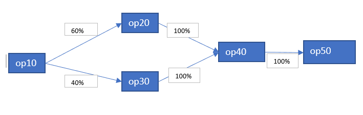
In Oracle Fusion Manufacturing, you can define operations with clear predecessor and successor relationships, enabling parallel operations. When creating a tactical plan, supply planning processes automatically take these dependencies into account to optimize material and resource allocation. This helps ensure accurate planning of both timing and quantities, resulting in more efficient and streamlined manufacturing operations.

Process Manufacturing

In process manufacturing, the calculation of component consumption, resource requirements, and co-product/by-product quantities are calculated independently of the transfer percentage maintained at each operation.
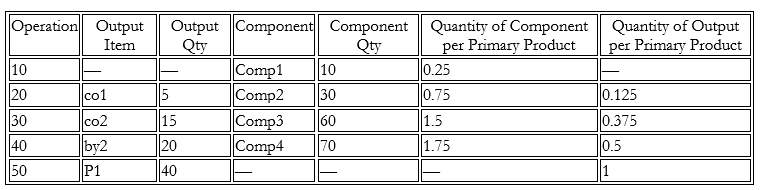
All quantities are treated with respect to the primary output quantity defined in the master data

process scm

Input Considerations

Primary Material (P1): 40 Units

Outputs by operation

Operation 20 --- Co-product co1 (5 Units)
Operation 30 --- Co-product co2 (15 Units)
Operation 40 --- By-product by2 (20 Units)
Operation 50 --- Primary Product P1 (40 Units)

Component Consumption by Operation

Operation 10 --- Comp1 (10 Units)
Operation 20 --- Comp2 (30 Units)
Operation 30 --- Comp3 (60 Units)
Operation 40 --- Comp4 (70 Units)

process scm 1

Key Interpretation

1. Quantity of Component per Primary Product

Formula:

Component Quantity ÷ Primary Product Quantity

Examples:

Comp2 --- 30 ÷ 40 = 0.75

2. Quantity of Output per Primary Product

Formula:

Output Quantity ÷ Primary Product Quantity

Examples:

co2 --- 15 ÷ 40 = 0.375

Without Yield Consideration

Supplies

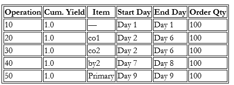
The primary product (P1) is completed at Operation 50.
Co-products (co1, co2) and a by-product (by2) are generated at intermediate operations.
The process spans Day 1 to Day 9 based on the resource usage at each operation and quantity to be processed at each operation.
The demand for Primary Product is 100 units.
Cumulative yield = 1 at all operations --- no losses assumed

process scm 2

Operation-Level Interpretation

Operation 10 (Day 1–Day 1)

Initial processing step with a start and output quantity of 100 units.
No co-product or by-product is generated at this stage.
The full batch is carried forward to subsequent operations.
Processing time is 1 day because the Resource(R1) usage is 0.24 hrs per unit. This means that 24 hrs. resource availability will be used while processing 100 units. Also, 24 hrs daily capacity is assumed for all the resources. Similarly, based on resource usage for specific resource at each operation processing time is calculated that is depicted in the resource requirements table.

Operation 20 (Day 2–Day 6)

Generates co-product (co1) with a quantity of 12.5 units, calculated as:
Quantity of Output per Primary Product × operation output quantity = 0.125 × 100
This output is proportionally derived from the total process quantity.
It is planned as a separate co-product without impacting the primary quantity.
Processing time is 5 days.
Based on transfer percentage defined at operation 20, 60% of the material gets transferred to operation 20.

Operation 30 (Day 2–Day 6)

Produces co-product (co2) with a quantity of 37.5 units, calculated as:
Quantity of Output per Primary Product × operation output quantity = 0.375 × 100

Occurs in parallel with Operation 20 within the same time frame.
Processing time is 4 days but still operation 30 is spanning across Day 2 to Day 6 because operation 20 and operation 30 in parallel are considered to be treated as in group.
Based on transfer percentage defined at operation 30, 40% of the material gets transferred to operation 30.

Operation 40 (Day 7–Day 8)

Generates by-product (by2) with a quantity of 50 units calculated as:
Quantity of Output per Primary Product × operation output quantity = 0.5 × 100
Processing time is 2 days and both parallel operation merge at operation 40.

Operation 50 (Day 9–Day 9)

Final production stage delivering 100 units of the primary product calculated as:
Quantity of Output per Primary Product × operation output quantity = 1 × 100

Processing time is 1 day.
Confirms that the process maintains full quantity consistency throughout.

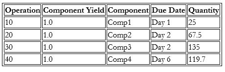
Component Requirement

The following table represents the operation-wise component consumption plan, where all components are assumed to have a yield factor of 1.0, meaning no losses are considered during consumption.

process scm 3

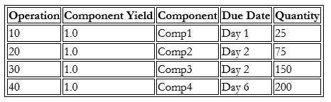
Component Consumption

Each operation is assigned a defined component requirement that is used during production execution without accounting for the transfer percentage between parallel operations.

The calculation is as follows:

Component quantity per primary product × operation input quantity (ignoring transfer percentage)

For example, for Comp2 on Day 2:
0.75 × 100 = 75 units

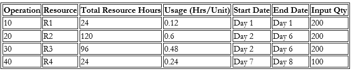
Resource Requirements

The table represents the operation-wise allocation of production resources (work centers) along with the associated capacity consumption in hours, based on a scheduled quantity of 100 units per operation.

process scm 4

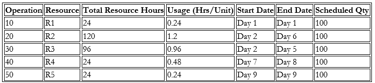
Each operation is assigned a resource that is utilized during production execution, without considering the transfer percentage across parallel operations.

The calculation is as follows:
Total Resource Hours = Usage (hrs/unit) × Input Quantity without transfer percentage

For example, for Resource (R2) on Day 2:
1.2 × 100 = 120 hours

This indicates:

Parallel processing (Operations 20 & 30 overlap) with each operation resource loading spanning across to its specific resource usage.
Sequential flow in later stages.
Capacity usage is directly proportional to production quantity.

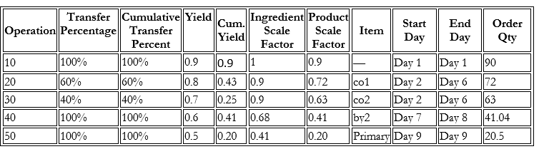
Yield Consideration

When Operation yield is maintained:

Yield is determined based on:
- Operation yield
- Transfer percentage between operations
The system calculates a cumulative yield factor across operations.
Product scale factors are determined based on operation yield defined till that operation.
Co-product/by-product quantities are then adjusted proportionally based on Product Scale Factor at each operation.
Component consumption, resource requirements are then adjusted proportionally based on Ingredient Scale Factor at each operation.

The system determines Product Scale Factor and Ingredient Scale Factor as follows:

Product Scale factor

Formula

PSFn equal to CYn / CTn

CYn equal to summation ( CYp* Yn * Tpn )

CTn equal to summation ( CTp * Tpn)

where,

CYn = Cumulative Yield at operation n
CYp = Cumulative Yield of the previous operation(s) leading into operation n
Yn = Operation yield at operation n
Tpn = Transfer percentage from previous operation p to operation n
PSFn = Product Scale factor for operation n
CTn = Cumulative Transfer Percent for operation n
CTp = Cumulative Transfer Percent for previous dependency operation

Ingredient Scale Factor

Formula

ISFn equal to CYn/(Yn * CTn)

where,

ISFn = Ingredient scale factor for operation n
CYn = Cumulative yield at operation n
Yn = Operation yield at operation n
CTn = Cumulative Transfer Percent for operation n

Supplies

The primary product (P1) is completed at Operation 50.
Co-products (co1, co2) and a by-product (by2) are generated at intermediate operations.
The process spans Day 1 to Day 9.
The demand for Primary Product is 20.5 units.
Operation yield present at all operations and losses are assumed.

process scm 5

Operation-Level Interpretation

Operation 10 (Day 1–Day 1)

Initial processing step with a start and output quantity of 100 units.
No co-product or by-product is generated at this stage.
The full batch is not carried forward to subsequent operations. Only 90 units move to operation 20.
Processing time is 1 day.

Operation 20 (Day 2–Day 6)

Generates co-product (co1) with a quantity of 9 units, calculated as:
Quantity of Output per Primary Product × operation output quantity = 0.125 × 72
This output is proportionally derived from the total process quantity.
It is planned as a separate co-product without impacting the primary quantity.
Processing time is 5 days.
Based on transfer percentage defined at operation 20, 60% of the material gets transferred to operation 20.

Operation 30 (Day 2–Day 6)

Produces co-product (co2) with a quantity of 23.62 units, calculated as:
Quantity of Output per Primary Product × operation output quantity = 0.375 × 63
Occurs in parallel with Operation 20 within the same time frame.
Processing time is 4 days but still operation 30 is spanning across Day 2 to Day 6 as operation 20 and operation 30 been parallel are treated as a group.
Based on transfer percentage defined at operation 30, 40% of the material gets transferred to operation 30.

Operation 40 (Day 7–Day 8)

Generates by-product (by2) with a quantity of 20.5 units calculated as:
Quantity of Output per Primary Product × operation output quantity = 0.5 × 41.04
Processing time is 2 days and both parallel operation merge at operation 40.
Cumulative Yield (Op40) = Cumulative Yield (Op20)*Yield(Op40)*Transfer Percentage(Op20 to Op40) + Cumulative Yield (Op30)*Yield(Op40)*Transfer Percentage(Op30 to Op40) = 43%*60%*100%+25%*60%*100%=41%.
Cumulative Transfer Percentage (Op40) = Cumulative Transfer Percentage (Op20) * Transfer Percentage (Op20 to Op40) + Cumulative Transfer Percentage (Op30) * Transfer Percentage (Op30 to Op40) = 60%*100% + 40%*100% = 100%.

Operation 50 (Day 9–Day 9)

Final production stage delivering 20.5 units of the primary product calculated as:
Quantity of Output per Primary Product × operation output quantity = 1 × 20.5
Processing time is 1 day.

Component Requirement

The following table represents the operation-wise component consumption plan, where all components are assumed to have a yield factor of 1.0, meaning no losses are considered during consumption.

process scm 6

Each operation is assigned a defined component requirement, which is used during production execution without accounting for the transfer percentage between parallel operations.

The calculation is as follows:

Component quantity per primary product × Ingredient Scale Factor * Start Quantity

Start Quantity = Demand/Cumulative Yield of last operation

For example, for Comp2 on Day 2:
0.75 × 0.9× 100 = 67.5 units

Resource Requirements

process scm 7

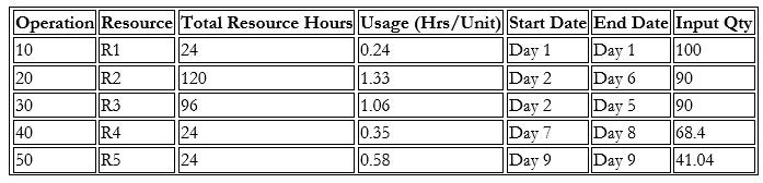
Each operation is assigned a resource that is utilized during production execution, without considering the transfer percentage across parallel operations.

The calculation is as follows:
Total Resource Hours = Usage (hrs/unit) × Input Quantity

Input Qty = Ingredient Scale Factor * Start Quantity

Start Quantity = Demand/Cumulative Yield of last operation

For example, for Resource (R2) on Day 2:
1.33 × 90 = 120 hours

This indicates:

Parallel processing (Operations 20 & 30 overlap) with each operation resource loading spanning across its specific resource usage.
Sequential flow in later stages.
Capacity usage is directly proportional to production quantity.

Discrete Manufacturing

In discrete manufacturing, the calculation of component consumption, resource requirements, and co-product or by-product quantities generally assumes that there is 100% transfer percentage between parallel operations. Finish-to-Start relationships between operations are primarily used in discrete manufacturing routing logic. Minimum yield defined across parallel operation is considered.

discrete scm

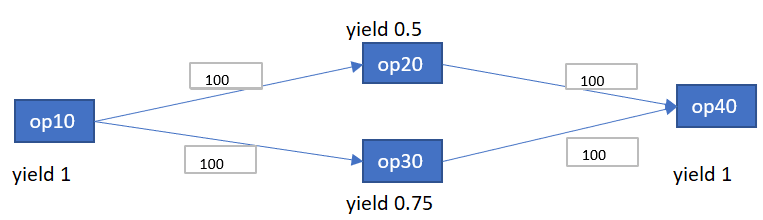
Input Considerations

Primary Material (P1): 40 Units

Outputs by Operation

Operation 30 --- By-product by2 (15 Units)
Operation 40 --- Primary Product P1 (40 Units)

Component Consumption by Operation

Operation 10 --- Comp1 (10 Units)
Operation 20 --- Comp2 (30 Units)
Operation 30 --- Comp3 (60 Units)

discrete scm 1

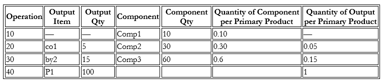
Key Interpretation

1. Quantity of Component per Primary Product

Formula:

Component Quantity ÷ Primary Product Quantity

Examples:

Comp2 --- 30 ÷ 100 = 0.30

2. Quantity of Output per Primary Product

Formula:

Output Quantity ÷ Primary Product Quantity

Examples:

by2 --- 15 ÷ 100 = 0.15

Supplies

The primary product (P1) is completed at Last Operation 40.
By-product (by2) is generated at intermediate operations.
The process spans Day 1 to Day 8.
The demand for Primary Product is 100 units.
Cumulative yield present at parallel operations and losses are assumed.

discrete scm 2

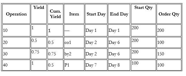
Operation-Level Interpretation

Operation 10 (Day 1–Day 1)

Initial processing step with a start and output quantity of 200 units.
No co-product or by-product is generated at this stage.
The full batch is carried forward to subsequent operations. 200 units moves to operation 20 and operation 30.
Processing time is 1 day.

Operation 20 (Day 2–Day 6)

Processing time is 5 days.
The whole quantity (100 units) moves to operation 20 from operation 10.

Operation 30 (Day 2–Day 6)

Produces co-product (co2) with a quantity of 22.5 units, calculated as:
Quantity of Output per Primary Product × operation output quantity = 0.15 × 150
Occurs in parallel with Operation 20 within the same time frame.
Processing time is 4 days but still operation 30 is spanning across Day 2 to Day 6 as operation 20 and operation 30 in parallel are treated as a group.
The whole quantity (100 units) moves to operation 20 from operation 10.

Operation 40 (Day 7–Day 8)

Generates by-product (by2) with a quantity of 100 units calculated as:
Quantity of Output per Primary Product × operation output quantity = 1 × 100
Processing time is 2 days and both parallel operation merge at operation 40.

Component Requirement

The following table represents the operation-wise component consumption plan, where all components are assumed to have a yield factor of 1.0, meaning no losses are considered during consumption.

discrete scm 3

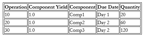
Each operation is assigned a defined component requirement that is used during production execution between parallel operations.

The calculation is as follows:

Component quantity per primary product × operation input quantity

For example, for Comp3 on Day 2:
0.6 × 200 = 120 units

Resource Requirements

discrete scm 4

Each operation is assigned a resource that is utilized during production execution across parallel operations.

The calculation is as follows:
Total Resource Hours = Usage (hrs/unit) × Input Quantity

For example, for Resource (R2) on Day 2:
0.6 × 200 = 120 hours

This indicates:

Parallel processing Operations 20 and 30 overlap with each operation resource loading spanning across to its specific resource usage.
Resource (R3) at operation 30 is spread across 5 days even if actual processing time for it is only 4 days due to operation 20 parallel setup.
Sequential flow in later stages.
Capacity usage is directly proportional to production quantity.

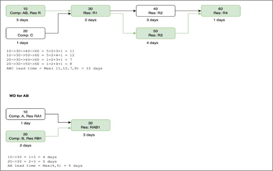
Lead time Calculation

Lead time for parallel operation takes the maximum possible total processing time for making the item in a work definition for all the combinations of paths taken into consideration. In other words, for parallel operations maximum lead time across parallel operation is considered.

For example, in the given screenshot it is 12 days for all the combination of route of the item.

Caption: Lead Time Calculation

Lead Time Calculation

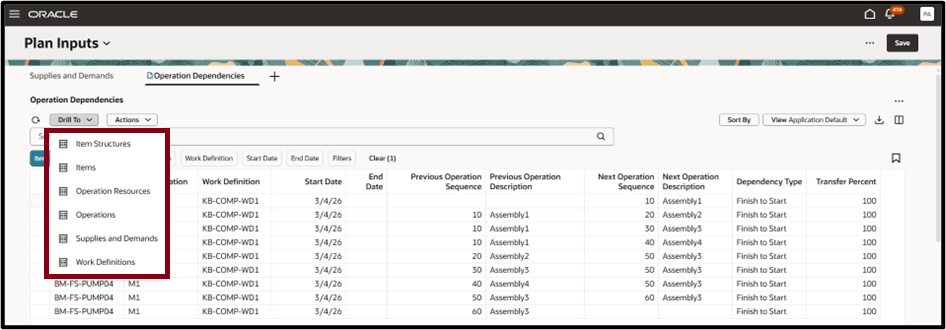
You can now define the parallel setup across operations within a work definition for both process and discrete manufacturing in Fusion or FBDI source. The Operation Dependencies page shows the setup across operation with corresponding dependency type and transfer percent as shown in the following screenshot.

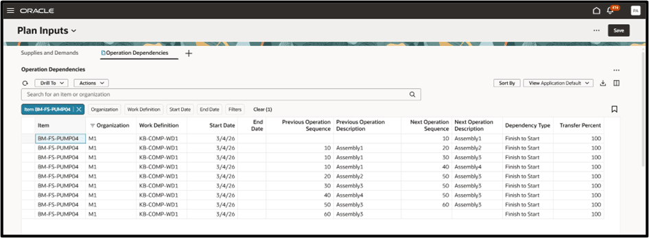
Operation Dependencies Page

You can drill from the Operation Dependencies page to the following seeded page with the following context:

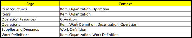
Drill to Context from Operation Dependencies Page

Drill to Seeded Page from Operation Dependencies Page

The operation dependencies are date effective.

Each Work Definition version duplicates the operation dependencies.
Operation dependencies can be modified at any time if the work definition version is effective on current or future date.
Deleting an operation in a work definition version also deletes any operation dependencies related to that operation in that version.
The following Operation Dependencies are supported:
- Finish to Start: Indicates that the previous operation must complete before the next operation can start. The completed quantity from the previous operation moves to the next operation. Transfer Percent is used to decide the amount of completed quantity to move.
- Start to Start: Indicates that the previous operation must start before the next operation can start. This is a purely scheduling dependency. There is no completed quantity movement from the previous to next operation.
- Interpretations while defining first and last operation:
  - First Operation: An operation with NULL previous operations. There must be at least 1 start operation, but there can be multiple first operations.
  - Last Operation: An operation with NULL next operation. There can be only one last operation.

For Planning, operations defined within a parallel setup are considered to be part of one group or set.

Steps to enable and configure

You don't need to do anything to enable this feature.

Access requirements

Users who are assigned a configured job role that contains these privileges can access this feature:

Monitor Demand and Supply Planning Work Area (MSC_MONITOR_DEMAND_AND_SUPPLY_PLANNING_WORK_AREA_PRIV)
Monitor Supply Planning Work Area (MSC_MONITOR_SUPPLY_PLANNING_WORK_AREA_PRIV)
View Planning Routings (MSC_VIEW_PLANNING_ROUTINGS_PRIV)

This privilege was available prior to this update.