3.4 Time Series Use Case
You work in an electronic store, and sales of laptops and tablets have increased over the last two quarters. You want to forecast your product sales for the next four quarters using historical timestamped data. You forecast sales using the Exponential Smoothing algorithm, predicting changes over evenly spaced intervals of time using historical data.
Table 3-2 Related Content
| Topic | Link |
|---|---|
| OML4Py GitHub Example | Time Series - Exponential Smoothing |
| About Time Series | About Time Series |
| About Model Setting | About Model Setting |
| Shared Settings | Shared Settings |
| Time Series Algorithm | Time Series Algorithm |
Before you start your OML4Py use case journey, ensure that you have the following:
-
Data Set
The data set used for this use case is from the SH schema. The SH schema can be readily accessed in Oracle Autonomous Database. For on-premises databases, the schema is installed during the installation or can be manually installed by downloading the scripts. See Installing the Sample Schemas.
You will use the
SALEStable from theSHschema. You can access the table by running theSELECTstatements in OML Notebooks. -
Database
Select or create a database using one of the following options:
- Get your FREE cloud account. Go to https://cloud.oracle.com/database and select Oracle Database Cloud Service (DBCS), or Oracle Autonomous Database. Create an account and create an instance. See Autonomous Database Quick Start Workshop.
- Download the latest version of Oracle Database (on premises).
-
Machine Learning Tools
Use OML Notebooks for Oracle Autonomous Database.
Topics:
- Access Data
Access the data set from the SH Schema and explore the data to understand the attributes. - Explore Data
Explore the data to understand and assess the quality of the data. At this stage assess the data to identify data types and noise in the data. Look for missing values and numeric outlier values. - Build Model
To build a model using the time series data, use the Exponential Smoothing algorithm on the OML proxy object ESM_SH_DATA generated during the exploratory stage. - Evaluate
Evaluate your model by viewing diagnostic metrics and performing quality checks.
Related Topics
Parent topic: Use Cases
3.4.1 Access Data
Access the data set from the SH Schema and explore the data to understand the attributes.
Remember:
The data set used for this use case is from the SH schema. The SH schema can be readily accessed in Oracle Autonomous AI Database. For on-premises databases, the schema is installed during the installation or can be manually installed by downloading the scripts. See Installing the Sample Schemas.
- Access the data.
- Examine the various attributes or columns of the data set.
- Assess data quality (by exploring the data).
Access Data
You will use SALES table data from the SH schema.
Examine Data
The following table displays information about the attributes from
SALES:
| Attribute Name | Information |
|---|---|
PROD_ID |
The ID of the product |
CUST_ID |
The ID of the customer |
TIME_ID |
The timestamp of the purchase of the product in yyy-mm-dd hh:mm:ss format |
CHANNEL_ID |
The channel ID of the channel sales data |
PROMO_ID |
The product promotion ID |
QUANTITY_SOLD |
The number of items sold |
AMOUNT_SOLD |
The amount or sales data |
Identify Target Variable
In this use case, the task is to train a model that predicts the amount sold.
Therefore, the target variable is the attribute AMOUNT_SOLD.
Parent topic: Time Series Use Case
3.4.2 Explore Data
Explore the data to understand and assess the quality of the data. At this stage assess the data to identify data types and noise in the data. Look for missing values and numeric outlier values.
Note:
Each record in the database is called a case and each case is identified
by a case_id. Here, the case id is TIME_ID, which
is an independent variable. You are forecasting the sales for evenly spaced
time.
The following steps help you with exploratory analysis of the data.
-
Import libraries
Run the following script in a
%pythoninterpreter paragraph to import theomlmodules, the Panda's module, and set the display options:import oml import pandas as pd import numpy as np import matplotlib.pyplot as plt pd.set_option('display.max_rows', 500) pd.set_option('display.max_columns', 500) pd.set_option('display.width', 1000) import warnings warnings.simplefilter(action='ignore', category=FutureWarning) -
Create a DataFrame proxy object on the SH.SALES table
Use theoml.syncfunction to create the Python object SALES as a proxy for a database table SALES. Theoml.syncfunction returns anoml.DataFrameobject.Note:
Only one environment for a given database schema can exist at a time. If"schema=None", then objects are created searched in the current user's schema.SALES = oml.sync(table = "SALES", schema = "SH") z.show(SALES.head())
-
Sales dataset row and column Count
To determine the number of rows and columns in the
oml.DataFrameobject SALES, useDataFrame.shape.print(f"Rows: {SALES.shape[0]}, Columns: SALES.shape[1]}")Rows: 918843, Columns: 7 -
Sales Dataset Column Types
Run the following script to view the data type of each column.print(f"Data types of each column in the Sales dataset:\n{SALES.dtypes}")
-
Count of missing values by column
To check if there are any missing values run the following script. The count function returns the number of elements that are not NULL for each column and the
len()function returns the number of rows in the dataset.print("Number of missing values in each column is : \n") print(len(SALES)-SALES.count())
-
Prepare data to forecast sales by selecting needed columns and view content
Now, prepare a Python proxy object called
ESM_SH_DATAby selecting the necessary columns fromSH.SALEStable. For this use case, selectTIME_IDandAMOUNT_SOLD.ESM_SH_DATA= SALES[['TIME_ID', 'AMOUNT_SOLD']] z.show(ESM_SH_DATA.head())
-
ESM_SH_DATA rows and columns
Determine the shape of
ESM_SH_DATA:print(f"Rows: {ESM_SH_DATA.shape[0]}, Columns: ESM_SH_DATA.shape[1]}")Rows: 918843, Columns: 2
This completes the data exploration stage.
Parent topic: Time Series Use Case
3.4.3 Build Model
To build a model using the time series data, use the Exponential Smoothing algorithm on the OML proxy object ESM_SH_DATA generated during the exploratory stage.
Oracle provides the Exponential Smoothing algorithm for time series.
Exponential smoothing is a forecasting method for time series data. It is a moving average method where exponentially decreasing weights are assigned to past observations. Components of Exponential Smoothing Model (ESM) such as trend and seasonality extensions, can have an additive or multiplicative form. For additive forms, the amplitude of the variation is independent of the level, whereas for multiplicative forms, the variation is connected to the level. The simpler additive models assume that error or noise, trend, and seasonality are linear effects within the recursive formulation.
To build a model using a supervised learning algorithm you may use a subset of the data into training and test data. Time series models usually use historical data to predict the future. This is different from model validation for classification and regression, which normally involves splitting data randomly into training and test sets. In this use case, there is no need to split the data set because the model is always predicting the current value based on information from the past. This means that although it seems that you train and test on the same data set, but when the model is applied, the forecast is always based on the previous date. In this use case, you will use the oml proxy object ESM_SH_DATA.
- To get help on the Exponential Smoothing Model (ESM), run the following
script:
help(oml.esm) - Create a Holt-Winters Model using quarterly setting
To build the model using the
ESM_SH_DATAproxy object, run the following statement:try: oml.drop(model = 'ESM_SALES_FORECAST_1') except: pass setting = {'EXSM_INTERVAL':'EXSM_INTERVAL_QTR', # accumulation interval = quarter 'EXSM_PREDICTION_STEP': '4', # prediction step = 4 quarters 'EXSM_MODEL': 'EXSM_WINTERS', # ESM model = Holt-Winters 'EXSM_SEASONALITY': '4', # seasonal cycle = 4 quarters 'EXSM_SETMISSING': 'EXSM_MISS_AUTO'} # treat missing values as an irregular time series train_x=ESM_SH_DATA[:,0] train_y=ESM_SH_DATA[:,1] esm_mod = oml.esm(**setting).fit(train_x, train_y, time_seq = 'TIME_ID')Examine the script:
EXSM_INTERVAL: Specifies the interval of the data set or a unit of interval size, like day, week, month, etc. This setting applies only to the time column with datetime type. For example, if you want to predict for quarterly sales, the setting isEXSM_INTERVAL_QTR.EXSM_PREDICTION_STEP: Specifies how many predictions to make. For example, if you want to display each value representing a quarter, then a value of 4 gives four values (Quarters) prediction into the future.EXSM_MODEL: Specifies the type of exponential smoothing model to be used. As an example, EXSM_WINTERS represents the Holt-Winters triple exponential smoothing model with additive trend and multiplicative seasonality. This type of model considers various combinations of additive and multiplicative trend, seasonality and error, with and without trend damping.EXSM_SEASONALITY: Specifies how long a season lasts. The parameter specifies a positive integer value as the length of seasonal cycle. The value it takes must be larger than 1. For example, 4 means that every group of four values forms a seasonal cycle, which makes sense if you are using 4 quarters to represent a year.EXSM_SETMISSING: Specifies how to handle missing values. In time series, the special value EXSM_MISS_AUTO indicates that, if the series contains missing values it is to be treated as an irregular time series.
This completes the model building stage.
Parent topic: Time Series Use Case
3.4.4 Evaluate
Evaluate your model by viewing diagnostic metrics and performing quality checks.
Sometimes querying dictionary views and model detail views is sufficient to measure your model's performance. However, you can evaluate your model by computing test metrics such as conditional log-likelihood, Average Mean Squared Error (AMSE), Akaike Information Criterion (AIC), and so on.
Information about Model settings
Evaluate the model by examining the various statistics generated after building the model. The statistics indicate the model's quality.
-
Review the forecast model settings
Run the following script for model details available through the GLM model object, like the model settings, attribute coefficients, fit details, etc.
z.show(ESM_MOD)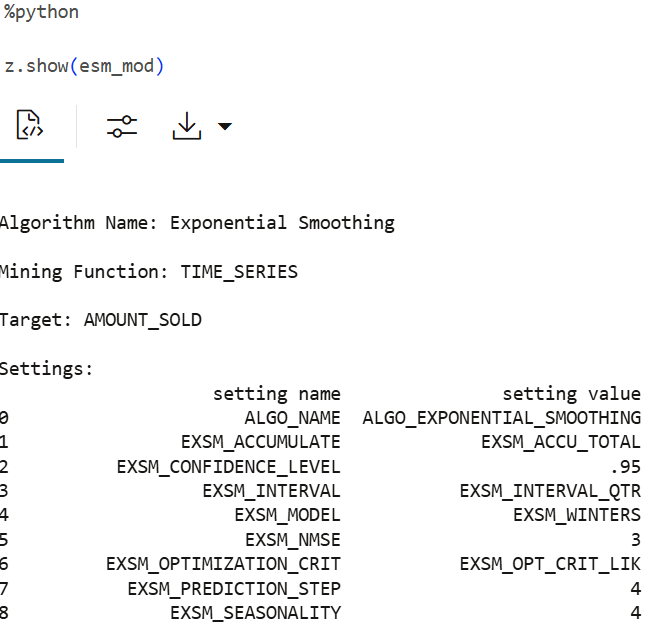
-
Review global diagnostics and model quality
Review the global diagnostics and model settings: Run the following script to display the model's global statistics.
z.show(ESM_MOD.global_stats)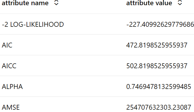
The attributes shown above are:
-2 Log_LIKELIHOOD: It is a statistical measure that evaluates how well a model fits the data. Specifically, it is calculated as twice the negative log-likelihood of the model. Generally, a lower value indicates a better-fit model. It’s often used to compare models, alongside criteria like AIC and BIC, for evaluating overall model performance.AIC: The Akaike Information Criterion (AIC) is used for model comparisions. It penalizes model complexity. Lower AIC indicates a better model.AICC: The Corrected Akaike Information Criterion (AICc) is a statistical measure used for model selection, particularly in the context of data analysis. It adjusts the Akaike Information Criterion (AIC) for small sample sizes, providing a more accurate estimate of the expected Kullback–Leibler discrepancy. The AICc is defined mathematically and is particularly useful when dealing with models that have a large number of parameters relative to the sample size.ALPHA: It is the smoothing parameter and ranges between 0 and 1. For exponential smoothing algorithm(Holt-Winters) it signifies the sensitivity of the forcast to recent changes in the data. Higher values indicate increased sensitivity.AMSE: AMSE, or Average Mean Squared Error measures the difference between the actual and forcasted value. It penalizes the higger errors. Lower AMSE values means better forcast accuracy.
Forecast
Here you will forecast sales for the next four quarters.
-
Forecast AMOUNT SOLD
The model, ESM_MOD, predicts 4 values into the future with LOWER and UPPER condifence bounds. The results are sorted by descending time sequence so that the latest points are shown first.
z.show(ESM_MOD.prediction.sort_values(by='TIME_SEQ',
          ascending=False))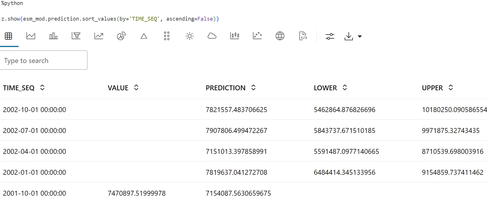
-
Chart forecasted AMOUNT_SOLD values with confidence intervals
To see a visual representation of the predictions in OML Notebooks, run the above same query with the following settings:
z.show(ESM_MOD.prediction.sort_values(by='TIME_SEQ'))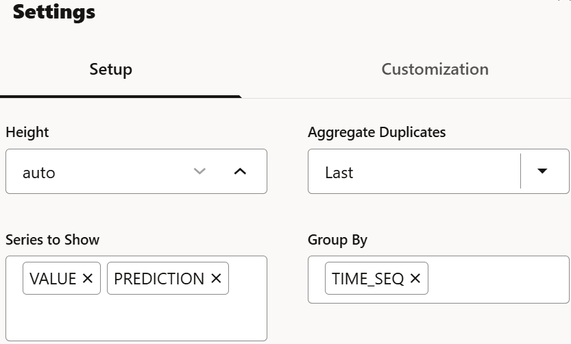
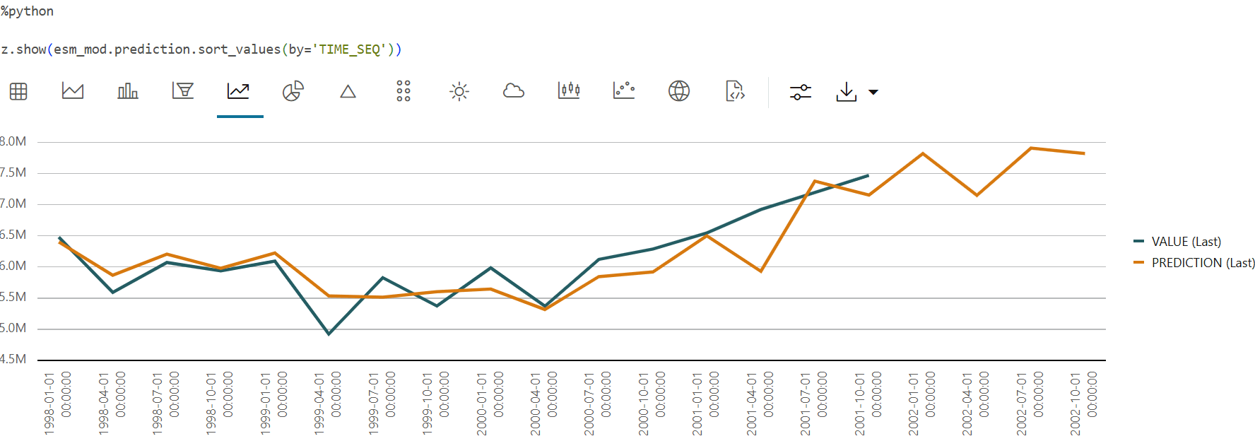
This completes the prediction step. The model has successfully forecast sales for the next four quarters. This helps in tracking the sales and also gives us an idea on stocking our products.
Parent topic: Time Series Use Case