Feature Extraction Use Case Scenario

You are developing a software application to recognize handwritten digits, which can be used to scan student answer sheets or forms. You are using the feature extraction technique to reduce the dimensionality of the dataset to produce a new feature space. This feature space concentrates the signal of the original data as linear combinations of the original data.

In other scenarios, feature extraction can be used to extract document themes, classify features, and so on.

The reduced features can be used with other machine learning algorithms, for example, classification and clustering algorithms.

In this use case, you'll use the neural network algorithm to recognize handwritten digits on the transformed space and contrast this with the accuracy using the original data.

You are using the default feature extraction algorithm Non-Negative Matrix Factorization (NMF) in two ways:

  1. Creating the Projections of the Top 16 Features, and feeding a Neural Networks (NN) model with those features
  2. Using the correlation between the various attributes and the Top 6 feature vectors to do an Attribute Selection manually and then feeding a Neural Network model with those features.

You are creating Neural Networks models to try to predict the correct handwritten digits based on an 8x8 image matrix (64 input attributes).

Related Content

Topic Link
OML4SQL GitHub Example Feature Extraction - Non-Negative Matrix Factorization
CREATE_MODEL2 Procedure CREATE_MODEL2 Procedure
Generic Model Settings DBMS_DATA_MINING - Model Settings
Non-negative Matrix Factorization (NMF) Settings DBMS_DATA_MINING - Algorithm Settings: Non-Negative Matrix Factorization
Data Dictionary Settings Oracle Machine Learning Data Dictionary Views
NMF - Model Detail Views Model Detail Views for Non-Negative Matrix Factorization
About Feature Extraction Feature Extraction
About NMF Non-Negative Matrix Factorization
About Classification Classification
About Neural Network Neural Network

Before you start your OML4SQL use case journey, ensure that you have the following:

Load Data

Create a table called DIGITS. This table is used to access the data set.

Perform these steps to load the data into your database.
  1. Download the DDL script, https://objectstorage.us-ashburn-1.oraclecloud.com/n/adwc4pm/b/OML_Data/o/digits.sql on your system.
  2. Open the file with a text editor and replace OML_USER02.DIGITS with <your username>.DIGITS. For example, if your OML Notebook account username is OML_USER, replace OML_USER02.DIGITS with OML_USER.DIGITS.
  3. Save the file.
  4. Copy the code and enter it into a notebook using OML Notebooks on ADB. Alternately, you can use Oracle SQL Developer with an on-premises Database or DBCS.
  5. Run the paragraph.
To understand the data, you will perform the following:
  • Access the data.
  • Examine the various attributes or columns of the data set.
  • Assess data quality (by exploring the data).

Examine Data

Digits data set has 64 numerical features or columns (8x8 pixel images). Each image is of a hand-written digit. The digits 0-9 are used in this data set.

Explore Data

Once the data is accessible, explore the data to understand and assess the quality of the data. .

Assess Data Quality

Because this is a well-curated data set, it is free of noise, missing values (systemic or random), and outlier numeric values.

The following steps help you with the exploratory analysis of the data:

  1. View the data in the DIGITS data by running the following statement:
    SELECT * FROM DIGITS;
  2. To see distinct data from the table, run the following query:
    SELECT DISTINCT * FROM DIGITS;
    View distinct data
  3. Find the COUNT of rows in the data set, run the following statement:
    SELECT COUNT(*) from DIGITS;
    COUNT(*)   
         1797 
    ---------------------------
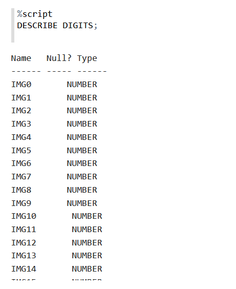
  4. To view the data type of the columns, run the following statement:
    %script
    DESCRIBE DIGITS;
    View the data type of the columns
  5. This SQL query will select the maximum, minimum, median, count, and mean of the "IMG59" column in the DIGITS table.
    The median value is calculated using the PERCENTILE_CONT function, which takes the percentile (in this case, the 50th percentile or median) as an argument.
    SELECT
        MAX(IMG59) as max_value,
        MIN(IMG59) as min_value,
        PERCENTILE_CONT(0.5) WITHIN GROUP (ORDER BY IMG59) as median_value,
        COUNT(*) as num_values,
        AVG(IMG59) as mean_value
    FROM DIGITS;
    Find the min, max, mean
  6. One way to find outliers is you can use the above query to calculate the mean and standard deviation of the data set, and then use those values to identify values that are outside of a certain number of standard deviations from the mean. Here, you are checking for one column - IMG59 mean and standard deviation.
    SELECT *
    FROM DIGITS
    WHERE 1.20 NOT BETWEEN (SELECT AVG(1.20) - 3 * STDDEV(1.20) FROM DIGITS)
    AND (SELECT AVG(1.20) + 3 * STDDEV(1.20) FROM DIGITS);
    Find outliers by checking the standard deviation from mean

This completes the data exploration stage. OML supports Automatic Data Preparation (ADP). ADP is enabled through the model settings. When ADP is enabled, the transformations required by the algorithm are performed automatically and embedded in the model. This step is done during the Build Model stage. The commonly used methods of data preparation are binning, normalization, and missing value treatment.

Build Model

Build your model using your data set. Use the DBMS_DATA_MINING.CREATE_MODEL2 procedure to build your model and specify the model settings.

Algorithm Selection

You can choose one of the following algorithms to solve a Feature Extraction problem:

  • Explicit Semantic Analysis (ESA) - this algorithm is not applicable for this use case data set.
  • Non-Negative Matrix Factorization (NMF)
  • Singular Value Decomposition (SVG)

Non-Negative matrix factorization (NMF) is now a popular tool for analyzing high-dimensional data because it automatically extracts sparse (missing values with mostly zero; many cells or pixels in this data set likely have zeros, however they are not truly missing) and meaningful features from a set of non-negative data vectors. NMF uses a low-rank matrix approximation to approximate a matrix X such that X is approximately equal to WH. The sub-matrix W contains the NMF basis column vectors; the sub-matrix H contains the associated coefficients (weights). The ability of NMF to automatically extract sparse and easily interpretable factors has led to its popularity. In the case of image recognition, such as digit images, the base images depict various handwritten digit prototypes and the columns of H indicate which feature is present in which image. Oracle Machine Learning uses NMF as the default algorithm for Feature Extraction.

For this use case, split the data into 60/40 as training and test data to further use it to compare the NMF model with that of another model using Neural Network (NN). You are splitting the data because you want to see how the model performs on data that you haven't seen before. If you put the whole data set into the original NMF model and then split it before giving it to NN, the NMF model has already seen the data when you try to test it. When we have completely new data, the extract features will not be based on it. You build the model using the training data and once the model is built, score the test data using the model.

The following steps guide you to build your model with the selected algorithm.

  1. To create the training and test data with 60/40 split, run the following statement:
    %script
    CREATE OR REPLACE VIEW TRAIN_DIGITS AS SELECT * FROM DIGITS SAMPLE (60) SEED (1);
    CREATE OR REPLACE VIEW TEST_DIGITS AS SELECT * FROM DIGITS MINUS SELECT * FROM TRAIN_DIGITS;
    
    View TRAIN_DIGITS created.
    
    ---------------------------
     
    View TEST_DIGITS created.
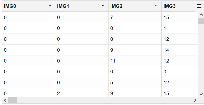
  2. To view the data in the TRAIN_DIGITS view, run the following statement:
    %sql
     
    SELECT * FROM TRAIN_DIGITS;
    View TRAIN_DIGITS table
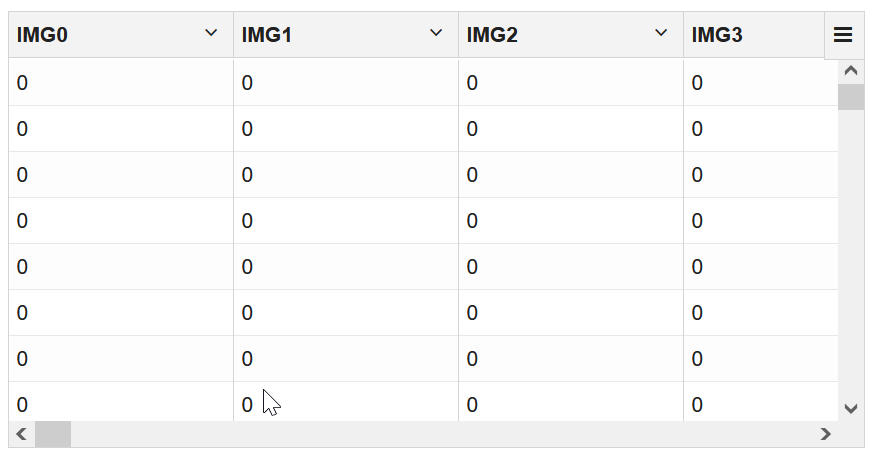
  3. To view the data in the TEST_DIGITS view, run the following statement:
    %sql
     
    SELECT * FROM TEST_DIGITS;
    View the TEST_DIGITS table
  4. To find the count of rows in TRAIN_DIGITS and TEST_DIGITS, run the following statement:
    %sql
    select 'TRAIN' dataset, count(*)  count from TRAIN_DIGITS
    union
    select 'TEST' dataset, count(*) count from TEST_DIGITS;
    Count of rows in TRAIN_DIGITS and TEST_DIGITS tables
  5. Build your model using the CREATE_MODEL2 procedure. First, declare a variable to store model settings or hyperparameters. Run the following script:
    %script
    BEGIN DBMS_DATA_MINING.DROP_MODEL('NMF_DIGITS');
    EXCEPTION WHEN OTHERS THEN NULL; END;
    /
    DECLARE
        v_setlst DBMS_DATA_MINING.SETTING_LIST;
        BEGIN
        v_setlst('PREP_AUTO') := 'ON';
        v_setlst('FEAT_NUM_FEATURES') := '16';
         
        DBMS_DATA_MINING.CREATE_MODEL2(
          MODEL_NAME          =>  'NMF_DIGITS',
          MINING_FUNCTION     => 'FEATURE_EXTRACTION',
          DATA_QUERY          =>  'SELECT * FROM DIGITS',
          CASE_ID_COLUMN_NAME =>  'TARGET'
          SET_LIST            =>  v_setlst);
    END;
    / 
    
    
    PL/SQL procedure successfully completed.
    ---------------------------
    PL/SQL procedure successfully completed.

    Examine the script:

    • v_setlist is a variable to store SETTING_LIST.
    • SETTING_LIST specifies model settings or hyperparameters for your model.
    • DBMS_DATA_MINING is the PL/SQL package used for machine learning. These settings are described in DBMS_DATA_MINING - Model Settings.
    • PREP_AUTO is the setting used for Automatic Data Preparation. Here, enable Automatic Data Preparation. The value of the setting is ON.
    • FEAT_NUM_FEATURES is the number of features you want to extract by using the feature extraction model. In this use case, 16 features are used for illustrative purposes.

    The CREATE_MODEL2 procedure takes the following parameters:

    • MODEL_NAME: A unique model name that you will give to your model. The name of the model is in the form [schema_name.]model_name. If you do not specify a schema, then your own schema is used. Here, the model name is NMF_DIGITS.
    • MINING_FUNCTION: Specifies the machine learning function or mining technique. Since in this use case you are performing feature extraction or dimensionality reduction, select the mining function as FEATURE_EXTRACTION.
    • DATA_QUERY: A query that provides training data for building the model. Here, the query is SELECT * FROM DIGITS.
    • SET_LIST: Specifies SETTING_LIST.
    • CASE_ID_COLUMN_NAME: A unique case identifier column in the build data. In this use case, case_id is CUST_ID. If there is a composite key, you must create a new attribute before creating the model. This may involve concatenating values from the columns, or mapping a unique identifier to each distinct combination of values. The CASE_ID assists with reproducible results, joining scores for individual rows with other data in, example, scoring data table. Here, since it an unsupervised technique, Target is unknown usually, here it is not required. So, to exclude it from processing, you are declaring it as case_id.

    Note:

    Any parameters or settings not specified are either system-determined or default values are used.

Evaluate

Evaluate your model by viewing diagnostic metrics and performing quality checks.

There is no specific set of testing parameters for feature extraction. In this use case, the evaluation mostly consists of comparing the NN models with and among the NMF models.

Dictionary and Model Views

To obtain information about the model and view model settings, you can query data dictionary views and model detail views. Specific views in model detail views display model statistics which can help you evaluate the model.

You'll be querying dictionary views. A database administrator (DBA) and USER versions of the views are also available. See Oracle Machine Learning Data Dictionary Views to learn more about the available dictionary views. Model detail views are specific to the algorithm. You can obtain more insights about the model you created by viewing the model detail views. The names of model detail views begin with DM$xx where xx corresponds to the view prefix. See Model Detail Views for more information.

The following steps help you to view different dictionary views and model detail views.

  1. Run the following statement to view the settings in USER_MINING_MODEL_SETTINGS:
    %script
     
    SELECT SETTING_NAME, SETTING_VALUE
      FROM USER_MINING_MODEL_SETTINGS
      WHERE MODEL_NAME='NMF_DIGITS'
      ORDER BY SETTING_NAME;


    SETTING_NAME                   SETTING_VALUE                   
    ALGO_NAME                      ALGO_NONNEGATIVE_MATRIX_FACTOR  
    FEAT_NUM_FEATURES              16                              
    NMFS_CONV_TOLERANCE            .05                             
    NMFS_NONNEGATIVE_SCORING       NMFS_NONNEG_SCORING_ENABLE      
    NMFS_NUM_ITERATIONS            50                              
    NMFS_RANDOM_SEED               -1                              
    ODMS_DETAILS                   ODMS_ENABLE                     
    ODMS_MISSING_VALUE_TREATMENT   ODMS_MISSING_VALUE_AUTO         
    ODMS_SAMPLING                  ODMS_SAMPLING_DISABLE           
    PREP_AUTO                      ON
    
    
    10 rows selected.
     
     
    --------------------------- 
    
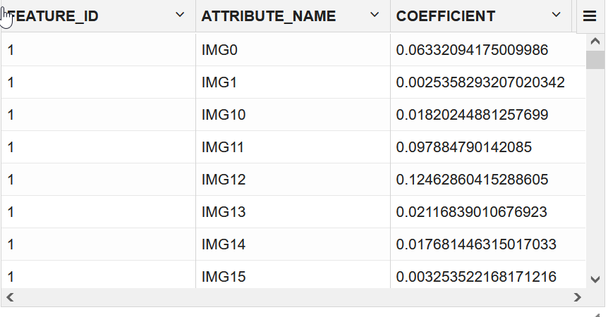
  2. The matrix of attribute values, or pixel values in this use case, is factored into two sub-matrices. Say the factorization is represented by the product of sub-matrices W and H, as WH. The sub-matrix H contains the coefficients (or weights) of the column vectors of sub-matrix W. To query the Non-Negative Matrix Factorization H Matrix, use the DM$VENMF view.
    %sql
    SELECT FEATURE_ID, ATTRIBUTE_NAME,
    ATTRIBUTE_VALUE, COEFFICIENT
    FROM DM$VENMF_DIGITS
    ORDER BY FEATURE_ID, ATTRIBUTE_NAME;  
    Outpout of model view DM$VENMF
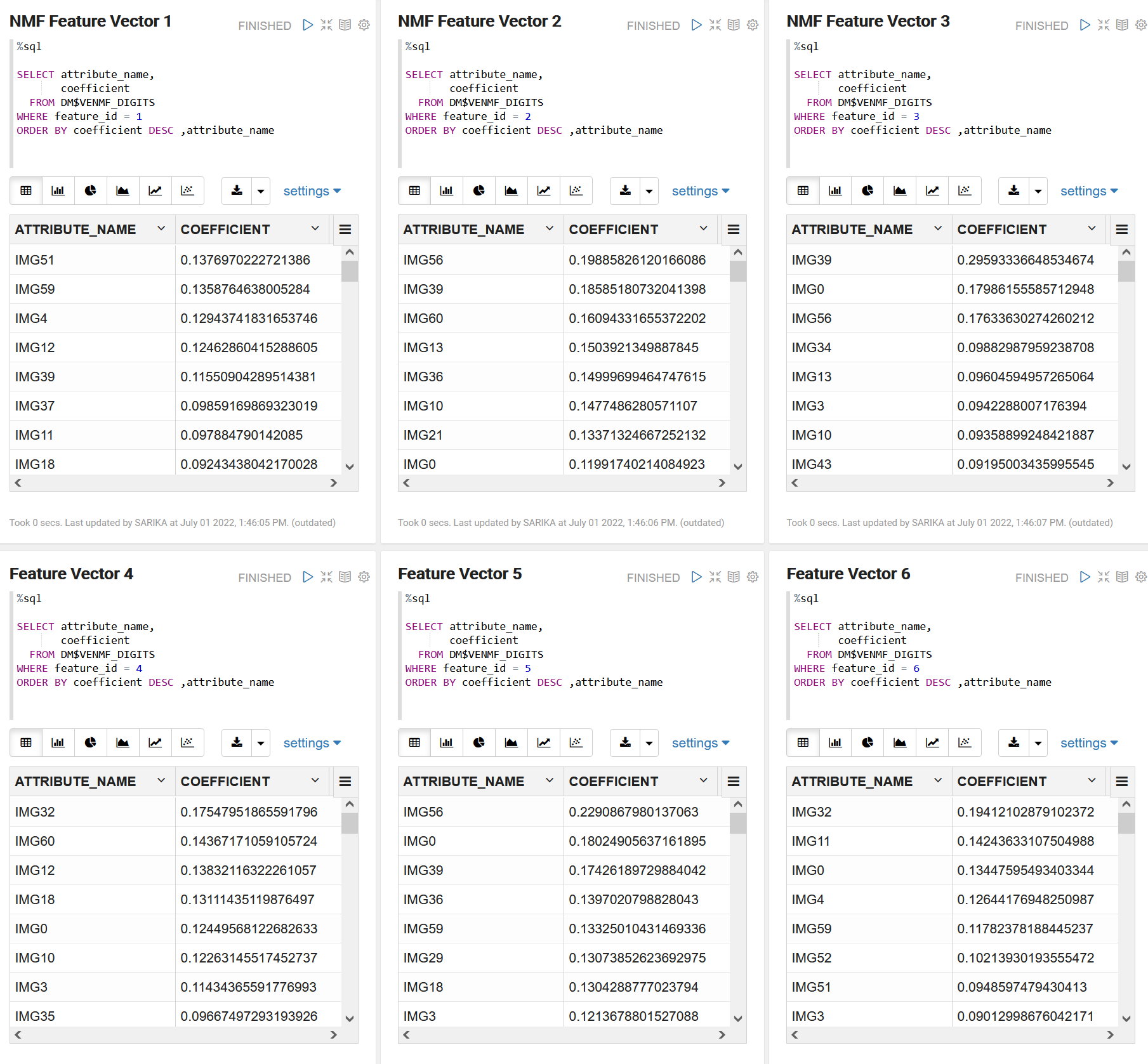
  3. Now, to understand the relationship between the original attribute set and the feature vectors, use the DM$VENMF view for each NMF feature vector. Each feature is a linear combination of the original attribute set. The coefficients of these linear combinations are non-negative. The model details return for each feature the coefficients associated with each one of the original attributes. This gives an idea of how the attributes are contributing to constructing each feature vector. For example, to view the attributes and coefficients for feature vector 1, use the WHERE clause and an ORDER BY clause in the query. Similarly, examine the attributes and their coefficients for feature vectors 2, 3, 4, 5, and 6 by changing the WHERE clause.
    %sql
     
    SELECT attribute_name,
           coefficient
      FROM DM$VENMF_DIGITS
    WHERE feature_id = 1
    ORDER BY coefficient DESC ,attribute_name 
    View thw coefficients associated with each of the original attributes for each feature vector
  4. Now, create another model using the Neural Network algorithm. You are first building a model with the original feature set (TRAIN_DIGITS) for comparison purposes before the extracted features are used.
    %script
     
    BEGIN DBMS_DATA_MINING.DROP_MODEL('NN_ORIG_DIGITS');
    EXCEPTION WHEN OTHERS THEN NULL; END;
    /
    DECLARE
        v_setlst DBMS_DATA_MINING.SETTING_LIST;
         
    BEGIN
        v_setlst('PREP_AUTO') := 'ON';
        v_setlst('ALGO_NAME') := 'ALGO_NEURAL_NETWORK';
        v_setlst('NNET_NODES_PER_LAYER') := '40';
        v_setlst('NNET_ACTIVATIONS') := '''NNET_ACTIVATIONS_TANH''';
        DBMS_DATA_MINING.CREATE_MODEL2(
            MODEL_NAME          => 'NN_ORIG_DIGITS',
            MINING_FUNCTION     => 'CLASSIFICATION',
            DATA_QUERY          => 'SELECT * FROM TRAIN_DIGITS',
            SET_LIST            => v_setlst,
            TARGET_COLUMN_NAME  => 'TARGET'
            );
             
    END;                             
     

    Examine the script:

    • v_setlist is a variable to store SETTING_LIST.
    • SETTING_LIST specifies model settings or hyperparameters for your model.
    • DBMS_DATA_MINING is the PL/SQL package used for machine learning. These settings are described in DBMS_DATA_MINING - Model Settings.
    • PREP_AUTO is the setting used for Automatic Data Preparation. Here, enable Automatic Data Preparation. The value of the setting is ON.
    • ALGO_NAME specifies the algorithm name. Since you are using the Neural Network as your algorithm, set ALGO_NEURAL_NETWORK.
    • NET_NODES_PER_LAYRER defines the topology by the number of nodes per layer. Different layers can have different numbers of nodes. To specify the same number of nodes for each layer, you can provide a single value, which is then applied to each layer. The default number of nodes per layer is the number of attributes or 50 (if the number of attributes > 50). In this use case, the defined value is 40, used for illustrative purposes.
    • NNET_ACTIVATIONS specifies the activation functions for the hidden layers. The activation function determines the output of neural networks. The activation functions map the outputs from a previous layer to values between 0 to 1 or -1 to 1, and so on, depending on the activation function applied. You can specify a single activation function, which is then applied to each hidden layer, or you can specify an activation function for each layer individually. See DBMS_DATA_MINING - Algorithm Settings: Neural Network to learn more about Neural Network settings. Different layers can have different activation functions. Here, you are using NNET_ACTIVATIONS_TANH. The range of the tanh function is from -1 to 1. The default value is the sigmoid function NNET_ACTIVATIONS_LOG_SIG, which has the range 0 to 1.

    The CREATE_MODEL2 procedure takes the following parameters:

    • MODEL_NAME: A unique model name that you will give to your model. The name of the model is in the form [schema_name.]model_name. If you do not specify a schema, then your own schema is used. Here, the model name is NN_ORIG_DIGITS.
    • MINING_FUNCTION: Specifies the machine learning function or mining technique. Since in this Since it is a Classification problem, for this model you selected CLASSIFICATION.
    • DATA_QUERY: A query that provides training data for building the model. Here, the query is SELECT * FROM TRAIN_DIGITS.
    • SET_LIST: Specifies SETTING_LIST.
    • TARGET_COLUMN_NAME: Specifies the column that needs to be predicted. Also referred to as the target variable of the model. In this use case, you are predicting the TARGET value.

    Note:

    Any parameters or settings not specified are either system-determined or default values are used.

Evaluate and Compare Models

You used the NMF feature extraction algorithm to transform your data and feed it into a NN model with the intention of improving predictive accuracy. You will now evaluate these classification models and compare the model accuracy.

You built a neural network classification model using the original data set, and then you used the data set transformed by the NMF model to build another neural network model. You will evaluate these classification models. When comparing these metrics, consider the model's quality by looking at prediction accuracy. Metrics can also be compared between models created by different feature extraction algorithms, the same extraction algorithm with different settings, or different classification algorithms and settings.

  1. To check if the model is converged, view the model views of the Neural Network model.

    %script
      SELECT VIEW_NAME, VIEW_TYPE
      FROM USER_MINING_MODEL_VIEWS
      WHERE MODEL_NAME='NN_ORIG_DIGITS'
      ORDER BY VIEW_NAME;
    
    VIEW_NAME             VIEW_TYPE                                 
    DM$VANN_ORIG_DIGITS   Neural Network Weights                    
    DM$VCNN_ORIG_DIGITS   Scoring Cost Matrix                       
    DM$VGNN_ORIG_DIGITS   Global Name-Value Pairs                   
    DM$VNNN_ORIG_DIGITS   Normalization and Missing Value Handling  
    DM$VSNN_ORIG_DIGITS   Computed Settings                         
    DM$VTNN_ORIG_DIGITS   Classification Targets                    
    DM$VWNN_ORIG_DIGITS   Model Build Alerts                        
     
     
    7 rows selected.
     
     
    ---------------------------
  2. Display the view DM$VGNN_ORIG_DIGITS to check the global name-value pairs to see if the model is converged which means that the model iterates until it reaches a point where no improvement in the result could be seen.

    %sql
     
    SELECT * from DM$VGNN_ORIG_DIGITS;
    View if the model is converged
  3. To check the quality of the model, run the following PCT accuracy code:

    %sql
     
    SELECT count(*) NUM_TEST_DIGITS,
           ROUND((SUM(CASE WHEN (TARGET - PRED_TARGET) = 0 THEN 1 ELSE 0 END)
                  / COUNT(*))*100,4) PCT_OVERALL_ACCURACY FROM
           (SELECT TARGET,
                   ROUND(PREDICTION(NN_ORIG_DIGITS USING *), 1) PRED_TARGET
                   FROM TEST_DIGITS)
    Check the overall accuracy of the model
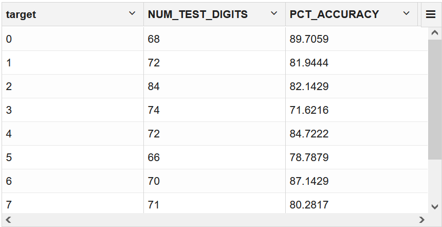
  4. To check the quality of the model per target digit, run the following PCT accuracy code:

    %sql
     
    SELECT TARGET,
           count(*) NUM_TEST_DIGITS,
           ROUND((SUM(CASE WHEN (TARGET - PRED_TARGET) = 0 THEN 1 ELSE 0 END)
                  / COUNT(*))*100,4) PCT_ACCURACY FROM
           (SELECT TARGET,
                   ROUND(PREDICTION(NN_ORIG_DIGITS USING *), 1) PRED_TARGET
                   FROM TEST_DIGITS)
            GROUP BY TARGET
            ORDER BY TARGET
    Check the accuracy per target digit
  5. To evaluate your model, use the following SQL PREDICTION function to generate a Confusion Matrix:
    %script
    SELECT "target" AS actual_target_value,
           PREDICTION(NN_ORIG_DIGITS USING *) AS predicted_target_value,
           COUNT(*) AS value
      FROM TEST_DIGITS
     GROUP BY "target", PREDICTION(NN_ORIG_DIGITS USING *)
     ORDER BY 1, 2;
    
    ACTUAL_TARGET_VALUE   PREDICTED_TARGET_VALUE   VALUE   
                        0                        0      81 
                        1                        1      83 
                        1                        8       1 
                        2                        1       1 
                        2                        2      72 
                        3                        2       1 
                        3                        3      68 
                        3                        5       1 
                        4                        4      65 
                        4                        7       1 
                        5                        5      63 
                        5                        6       1 
                        5                        7       1 
                        5                        9       1 
    
    ACTUAL_TARGET_VALUE   PREDICTED_TARGET_VALUE   VALUE   
                        6                        5       2 
                        6                        6      64 
                        7                        7      63 
                        7                        9       1 
                        8                        1       1 
                        8                        2       1 
                        8                        7       1 
                        8                        8      55 
                        8                        9       1 
                        9                        3       1 
                        9                        5       1 
                        9                        8       1 
                        9                        9      81 
    
    
    27 rows selected. 
    
    
    ---------------------------

Score

Scoring an NMF model produces data projections in the new feature space. The magnitude of a projection indicates how strongly a record maps to a feature.

In this use case, there are two options to produce projections to compare using the Neural Network model. One is to build a neural network model on the top 16 features of NMF to predict the digits. Another is to build a neural network model by manually selecting the original attributes with the highest coefficients for each feature vector.

For option one, create a new TRAIN and TEST view and then build a NN model.

  1. Create a new TRAIN view with the top 16 NMF features.
    %sql
     
    CREATE OR REPLACE VIEW TRAIN_NMF_FEATURES AS
    SELECT TARGET,
           FEATURE_VALUE(NMF_DIGITS, 1 USING *) PROJ1,
           FEATURE_VALUE(NMF_DIGITS, 2 USING *) PROJ2,
           FEATURE_VALUE(NMF_DIGITS, 3 USING *) PROJ3,
           FEATURE_VALUE(NMF_DIGITS, 4 USING *) PROJ4,
           FEATURE_VALUE(NMF_DIGITS, 5 USING *) PROJ5,
           FEATURE_VALUE(NMF_DIGITS, 6 USING *) PROJ6,
           FEATURE_VALUE(NMF_DIGITS, 7 USING *) PROJ7,
           FEATURE_VALUE(NMF_DIGITS, 8 USING *) PROJ8,
           FEATURE_VALUE(NMF_DIGITS, 9 USING *) PROJ9,
           FEATURE_VALUE(NMF_DIGITS, 10 USING *) PROJ10,
           FEATURE_VALUE(NMF_DIGITS, 11 USING *) PROJ11,
           FEATURE_VALUE(NMF_DIGITS, 12 USING *) PROJ12,
           FEATURE_VALUE(NMF_DIGITS, 13 USING *) PROJ13,
           FEATURE_VALUE(NMF_DIGITS, 14 USING *) PROJ14,
           FEATURE_VALUE(NMF_DIGITS, 15 USING *) PROJ15,
           FEATURE_VALUE(NMF_DIGITS, 16 USING *) PROJ16
    FROM TRAIN_DIGITS;
    
    TRAIN_DIGITS view created
    ---------------------------
  2. Create a new TEST view with the top 16 NMF features.
    %sql
     
    CREATE OR REPLACE VIEW TEST_NMF_FEATURES AS
    SELECT TARGET,
           FEATURE_VALUE(NMF_DIGITS, 1 USING *) PROJ1,
           FEATURE_VALUE(NMF_DIGITS, 2 USING *) PROJ2,
           FEATURE_VALUE(NMF_DIGITS, 3 USING *) PROJ3,
           FEATURE_VALUE(NMF_DIGITS, 4 USING *) PROJ4,
           FEATURE_VALUE(NMF_DIGITS, 5 USING *) PROJ5,
           FEATURE_VALUE(NMF_DIGITS, 6 USING *) PROJ6,
           FEATURE_VALUE(NMF_DIGITS, 7 USING *) PROJ7,
           FEATURE_VALUE(NMF_DIGITS, 8 USING *) PROJ8,
           FEATURE_VALUE(NMF_DIGITS, 9 USING *) PROJ9,
           FEATURE_VALUE(NMF_DIGITS, 10 USING *) PROJ10,
           FEATURE_VALUE(NMF_DIGITS, 11 USING *) PROJ11,
           FEATURE_VALUE(NMF_DIGITS, 12 USING *) PROJ12,
           FEATURE_VALUE(NMF_DIGITS, 13 USING *) PROJ13,
           FEATURE_VALUE(NMF_DIGITS, 14 USING *) PROJ14,
           FEATURE_VALUE(NMF_DIGITS, 15 USING *) PROJ15,
           FEATURE_VALUE(NMF_DIGITS, 16 USING *) PROJ16
    FROM TEST_DIGITS;
    
    TEST_DIGITS view created
    ---------------------------
  3. Build a Neural Network model using the new TRAIN data set.
    %script
     
    BEGIN DBMS_DATA_MINING.DROP_MODEL('NN_NMF_DIGITS');
    EXCEPTION WHEN OTHERS THEN NULL; END;
    /
    DECLARE
        v_setlst DBMS_DATA_MINING.SETTING_LIST;
         
    BEGIN
        v_setlst('PREP_AUTO') := 'ON';
        v_setlst('ALGO_NAME') := 'ALGO_NEURAL_NETWORK';
        v_setlst('NNET_NODES_PER_LAYER') := '40';
        v_setlst('NNET_ACTIVATIONS') := '''NNET_ACTIVATIONS_TANH''';   
        DBMS_DATA_MINING.CREATE_MODEL2(
            MODEL_NAME          => 'NN_NMF_DIGITS',
            MINING_FUNCTION     => 'CLASSIFICATION',
            DATA_QUERY          => 'SELECT * FROM TRAIN_NMF_FEATURES',
            SET_LIST            => v_setlst,
            TARGET_COLUMN_NAME  => 'TARGET'
            );
             
    END;
  4. Check the convergence of the model.
    %sql
     
    SELECT * from DM$VGNN_NMF_DIGITS;
    Check the convergence of a model
  5. Check the quality of the model using PCT accuracy.
    %sql
     
    SELECT count(*) NUM_TEST_DIGITS,
           ROUND((SUM(CASE WHEN (TARGET - PRED_TARGET) = 0 THEN 1 ELSE 0 END)
                  / COUNT(*))*100,4) PCT_OVERALL_ACCURACY FROM
           (SELECT TARGET,
                   ROUND(PREDICTION(NN_NMF_DIGITS USING *), 1) PRED_TARGET
                   FROM TEST_NMF_FEATURES)
    Observe the overall accuracy of the model

    Compare the overall accuracy of the model with the original dataset and the overall accuracy of the model with the top 16 NMF features.

    Tip:

    The overall accuracy score looks poor here. This is for illustrative purposes. You may consider increasing the number to top 32 NMF features. Alternately, you can try a different algorithm.
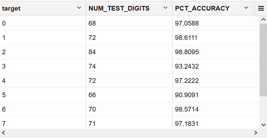
  6. Check the PCT accuracy of the target digit.
    %sql
     
    SELECT TARGET,
           count(*) NUM_TEST_DIGITS,
           ROUND((SUM(CASE WHEN (TARGET - PRED_TARGET) = 0 THEN 1 ELSE 0 END)
                  / COUNT(*))*100,4) PCT_ACCURACY FROM
           (SELECT TARGET,
                   ROUND(PREDICTION(NN_NMF_DIGITS USING *), 1) PRED_TARGET
                   FROM TEST_NMF_FEATURES)
            GROUP BY TARGET
            ORDER BY TARGET
    Observe the target digit accuracy
You'll notice that the model with the original dataset has better accuracy than the one with the top 16 NMF features. Further, let's see another model built by manually selecting the attributes for each feature vector having the highest coefficients and comparing the quality of all the models.

Score with Selected Attributes

You are creating another Neural Network model by manually selecting the attributes in each extracted feature vector based on their coefficients.

That means selecting all the unique attributes that have the highest coefficients with the feature vectors. Earlier you have seen the relationship of the original attributes and attribute coefficients with six feature vectors. See Step 3 of Dictionary and Model Views. For example, for Feature 1 select the following attributes: IMG51, IMG12, IMG59, IMG4, IMG27, IMG28, IMG44, IMG11, IMG37, IMG61, IMG50. The unique attributes for the six feature vectors are:
  • Feature 1: IMG51, IMG12, IMG59, IMG4, IMG27, IMG28, IMG44, IMG11, IMG37, IMG61, IMG50
  • Feature 2: IMG32, IMG39, IMG56, IMG0, IMG20, IMG19,
  • Feature 3: IMG18, IMG36, IMG26, IMG21, IMG42
  • Feature 4: IMG60, IMG3, IMG43, IMG34,
  • Feature 5: IMG53, IMG13, IMG58, IMG10
  • Feature 6: IMG29, IMG35, IMG52

Now create a new TRAIN and TEST view and then build a neural network model.

  1. Create a new TRAIN_NMF_ATTR view with the top unique attributes.
    %sql
     
    CREATE OR REPLACE VIEW TRAIN_NMF_ATTR AS
    SELECT TARGET,
           IMG51, IMG12, IMG59, IMG4, IMG27, IMG28, IMG44, IMG11, IMG37, IMG61, IMG50
           IMG32, IMG39, IMG56, IMG0, IMG20, IMG19,
           IMG18, IMG36, IMG26, IMG21, IMG42
           IMG60, IMG3, IMG43, IMG34,
           IMG53, IMG13, IMG58, IMG10,
           IMG29, IMG35, IMG52
    FROM TRAIN_DIGITS;
    
    TRAIN_NMF_ATTR view created
    ---------------------------
  2. Create a TEST_NMF_FEATURES view with the top unique attributes.
    %sql
     
    CREATE OR REPLACE VIEW TEST_NMF_ATTR AS
    SELECT TARGET,
           IMG51, IMG12, IMG59, IMG4, IMG27, IMG28, IMG44, IMG11, IMG37, IMG61, IMG50
           IMG32, IMG39, IMG56, IMG0, IMG20, IMG19,
           IMG18, IMG36, IMG26, IMG21, IMG42
           IMG60, IMG3, IMG43, IMG34,
           IMG53, IMG13, IMG58, IMG10,
           IMG29, IMG35, IMG52
    FROM TEST_DIGITS;
    
    TEST_NMF_FEATURES view created
    ---------------------------
  3. Build a Neural Network model using the new TRAIN_NMF_ATTR data set.
    %script
     
    BEGIN DBMS_DATA_MINING.DROP_MODEL('NN_NMF_ATT_DIGITS');
    EXCEPTION WHEN OTHERS THEN NULL; END;
    /
    DECLARE
        v_setlst DBMS_DATA_MINING.SETTING_LIST;
         
    BEGIN
        v_setlst('PREP_AUTO') := 'ON';
        v_setlst('ALGO_NAME') := 'ALGO_NEURAL_NETWORK';
        v_setlst('NNET_NODES_PER_LAYER') := '40';
        v_setlst('NNET_ACTIVATIONS') := '''NNET_ACTIVATIONS_TANH''';
        DBMS_DATA_MINING.CREATE_MODEL2(
            MODEL_NAME          => 'NN_NMF_ATT_DIGITS',
            MINING_FUNCTION     => 'CLASSIFICATION',
            DATA_QUERY          => 'SELECT * FROM TRAIN_NMF_ATTR',
            SET_LIST            => v_setlst,
            TARGET_COLUMN_NAME  => 'TARGET'
            );
             
    END;
    PL/SQL procedure successfully completed.
     
    ---------------------------
     
    PL/SQL procedure successfully completed.
  4. Check the convergence of the model.
    %sql
     
    SELECT * from DM$VGNN_NMF_ATT_DIGITS;
    Check for model convergence
  5. Check the quality of the model using PCT accuracy.
    %sql
     
    SELECT count(*) NUM_TEST_DIGITS,
           ROUND((SUM(CASE WHEN (TARGET - PRED_TARGET) = 0 THEN 1 ELSE 0 END)
                  / COUNT(*))*100,4) PCT_OVERALL_ACCURACY FROM
           (SELECT TARGET,
                   ROUND(PREDICTION(NN_NMF_ATT_DIGITS USING *), 1) PRED_TARGET
                   FROM TEST_NMF_ATTR)
    Observe the accuracy of the model

    Compare the overall accuracy of the model with manually selected attributes with those of the earlier models.

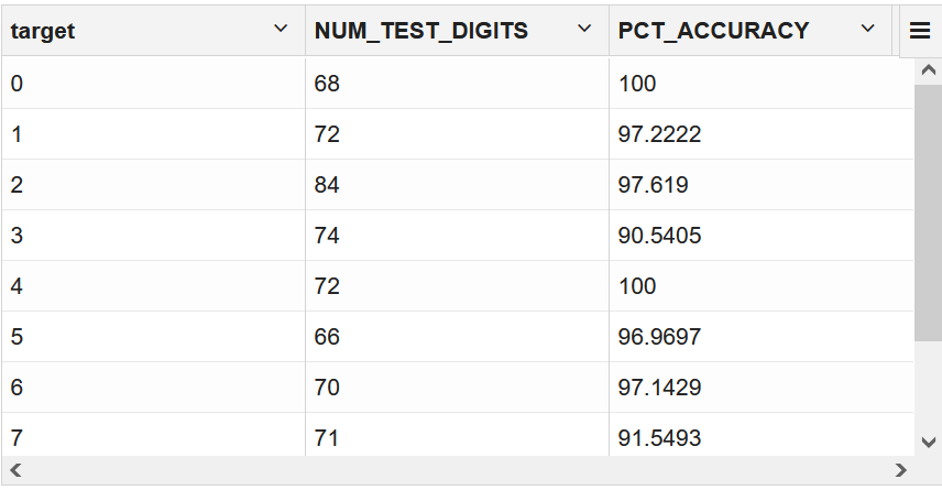
  6. Check the PCT accuracy of the target digit.
    %sql
     
    SELECT TARGET,
           count(*) NUM_TEST_DIGITS,
           ROUND((SUM(CASE WHEN (TARGET - PRED_TARGET) = 0 THEN 1 ELSE 0 END)
                  / COUNT(*))*100,4) PCT_ACCURACY FROM
           (SELECT TARGET,
                   ROUND(PREDICTION(NN_NMF_ATT_DIGITS USING *), 1) PRED_TARGET
                   FROM TEST_NMF_ATTR)
            GROUP BY TARGET
            ORDER BY TARGET
    Observe the target digit accuracy

Table 3-1 PCT Accuracy Comparison

Model NUM_TEST_DIGITS PCT_OVERALL_ACCURACY
NN model 1 with extracted features as input 725 96
NN model 2 with top 16 features of NMF data 725 79.4483
NN model 3 with original attributes with highest coeffient for each feature vector 725 96.1379

You found that the NN model using the 16 NMF Feature projections had a lower overall accuracy. However, the model using a reduced set of Attributes as input to the NN (using 33 out of the 64 total attributes, as suggested by NMF as being the most important) has shown a slightly better overall accuracy when compared to the original.

This way you can use one of these models for your app to read student sheets or forms to recognize handwritten numbers.