Dimensions and Members
If you understand dimensions and members, you are well on your way to understanding the power of a multidimensional database.
For example, Year is a dimension (of type Time) and Qtr1 is a member:
Year Time
   Qtr1 (+)
      Jan (+)
......Feb (+)
......Mar (+)
There are two types of dimensions: standard and attribute.
-
Standard dimensions represent the core components of a business plan and often relate to departmental functions. Typical standard dimensions: Time, Accounts, Product Line, Market, and Division. Dimensions change less frequently than members.
-
Attribute dimensions are associated with standard dimensions. Through attribute dimensions, you group and analyze members of standard dimensions based on the member attributes (characteristics). For example, you can compare the profitability of noncaffeinated products that are packaged in glass to the profitability of noncaffeinated products packaged in cans.
Members are the individual components of a dimension. For example, Product A, Product B, and Product C might be members of the Product dimension. Each member has a unique name. Data associated with a member can be stored (referred to as a stored member in this chapter), or the data can be dynamically calculated when a user retrieves it.
Outline Hierarchies
Start designing your Essbase cube by defining an outline. The outline organization reflects the relationship of your data categories as structural and mathematical hierarchies.
Essbase database (cube) development begins with creating an outline, which accomplishes the following objectives:
-
Defines structural relationships
-
Organizes data
-
Defines the consolidations and mathematical relationships between items
The concept of members is used to represent data hierarchies. Each dimension consists of one or more members. The members, in turn, may consist of other members. When you create a dimension, you define how to consolidate the values of its individual members. Within the tree structure of the cube outline, a consolidation is a group of members in a branch of the tree.
For example, many businesses summarize their data monthly, rolling up monthly data to obtain quarterly figures and rolling up quarterly data to obtain annual figures. Businesses may also summarize data by zip code, city, state, and country. Any dimension can be used to consolidate data for reporting purposes.
In the Sample.Basic cube, for example, the Year dimension includes quarter members: Qtr1, Qtr2, Qtr3, and Qtr4, each storing data for an individual quarter, and Year, storing summary data for the year. Qtr1 includes Jan, Feb, and Mar, each storing data for a month, and Qtr1, storing summary data for the quarter. Similarly, Qtr2, Qtr3, and Qtr4 include the members that represent the individual months, and the member that stores the quarterly totals.
The following hierarchical structure represents the data consolidations and relationships in Qtr1.
Year Time
   Qtr1 (+)
      Jan (+)
......Feb (+)
......Mar (+)
Some dimensions consist of relatively few members, while others may have hundreds or thousands of members.
Dimension and Member Relationships
The organization of an Essbase outline is described using hierarchical and familial terminology, as it's an easy way to conceptualize roles and relationships of members within a dimension. Hierarchical terms include generations and levels, which are analogous to roots and leaves. Familial terms include parents, children, siblings, descendants, and ancestors.
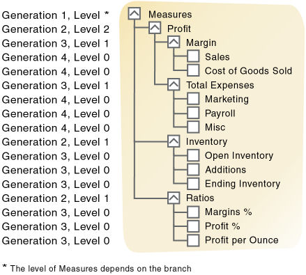
The subtopics in this section reference the outline shown below in describing the position of the members in the outline.
Figure 2-1 Member Generation and Level Numbers
Parents, Children, and Siblings
The outline illustrates the following parent, child, and sibling relationships:
-
A parent is a member that has a branch below it. For example, Margin is a parent member for Sales and Cost of Goods Sold.
-
A child is a member that has a parent above it. For example, Sales and Cost of Goods Sold are children of the parent Margin.
-
Siblings are child members of the same immediate parent, at the same generation. For example, Sales and Cost of Goods Sold are siblings (they both have the parent Margin), but Marketing (at the same branch level) is not a sibling, because its parent is Total Expenses.
Descendants and Ancestors
The outline illustrates the following descendant and ancestral relationships:
-
Descendants are members in branches below a parent. For example, Profit, Inventory, and Ratios are descendants of Measures. The children of Profit, Inventory, and Ratios are also descendants of Measures.
-
Ancestors are members in branches above a member. For example, Margin, Profit, and Measures are ancestors of Sales.
Roots and Leaves
The outline illustrates the following root and leaf member relationships:
-
The root is the top member in a branch. Measures is the root for Profit, Inventory, Ratios.
-
Leaf members have no children and are also referred to as level 0 members. For example, Opening Inventory, Additions, and Ending Inventory are level 0 members.
Generations and Levels
In Essbase, generations and levels are indicators about a member's place in the outline structure. A generation indicates the distance of a member from the root of the dimension. A level measures the number of branches between a member and the lowest member below it (a hierarchical "leaf").
Generations
Generation refers to a consolidation level within a dimension. A root branch of the tree is generation 1. Generation numbers increase as you count from the root toward the leaf member. In the outline, Measures is generation 1, Profit is generation 2, and Margin is generation 3. All siblings of each level belong to the same generation; for example, both Inventory and Ratios are generation 2.
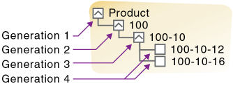
In the following illustration, part of the Product dimension is shown, with its generations numbered. Product is generation 1, 100 is generation 2, 100-10 is generation 3, and 100-10-12 and 100-10-16 are generation 4.
Figure 2-2 Generations
Levels
Level also refers to a branch within a dimension; levels reverse the numerical ordering used for generations. Levels count up from the leaf member toward the root. The root level number varies depending on the depth of the branch. In the outline illustration at the beginning of this section, Sales and Cost of Goods Sold are level 0. All other leaf members are also level 0. Margin is level 1, and Profit is level 2. Notice that the level number of Measures varies depending on the branch. For the Ratios branch, Measures is level 2. For the Total Expenses branch, Measures is level 3.
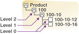
In the following illustration, part of the Product dimension is shown, with its levels numbered. 100 is level 2, 100-10 is level 1, and 100-10-12 and 100-10-16 are level 0.
Figure 2-3 Levels
Generation and Level Names
To ease report maintenance, you can assign a name to a generation or level and then use the name as a shorthand for all members in that generation or level. Because changes to an outline are automatically reflected in a report, when you use generation and level names, you do not need to change the report if a member name is changed or deleted from the database outline.
Hierarchy Shapes
Hierarchies in Essbase can be symmetric or asymmetric (ragged).
Essbase handles some operations differently depending on the hierarchy shape. Tabular data export, certain calculation functions (including @ANCESTVAL), and drill through report mapping can have different outcomes when a dimension contains asymmetric hierarchies.
Symmetric Hierarchies
In symmetric hierarchies, members with the same level number are at the same depth in the outline. For example, in the following diagram, members 100-10 and 200-10 are both level 0 members, and they are both generation 3 members:
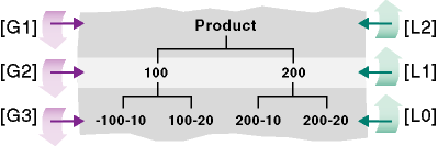
Generation numbers begin counting with 1 at the dimension name; higher generation numbers are those that are closest to leaf members in a hierarchy.
Level numbers begin with 0 at the deepest part of the hierarchy; the highest level number is a dimension name.
Asymmetric Hierarchies
In asymmetric (or ragged) hierarchies, having the same level number does not mean that members are at the same depth in the outline. For example, in the following diagram, member aa and member f are both level 0 members, and yet they are not at the same depth:

Standard Dimensions and Attribute Dimensions
Essbase has standard dimensions and attribute dimensions. This chapter focuses on standard dimensions, because Essbase does not allocate storage for attribute dimension members. Instead, it dynamically calculates the members when the user queries data associated with them.
An attribute dimension is a special type of dimension that is associated with a standard dimension. See Work with Essbase Attributes.
Sparse and Dense Dimensions
Most data sets of multidimensional databases have two characteristics:
-
Data is not smoothly and uniformly distributed.
-
Data does not exist for the majority of member combinations. For example, all products may not be sold in all areas of the country.
Most multidimensional databases are inherently sparse; they lack data values for the majority of member combinations. A sparse dimension is one with a low percentage of available data positions filled.
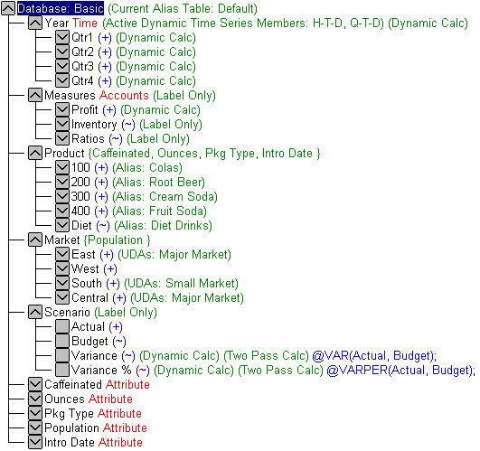
For example, the outline of the Sample.Basic database in Figure 2-4 includes the Year, Product, Market, Measures, and Scenario dimensions. Product represents the product units, Market represents the geographical regions in which the products are sold, and Measures represents the accounts data. Because not every product is sold in every market, Market and Product are chosen as sparse dimensions.
Multidimensional databases also contain dense dimensions. A dense dimension has a high probability that one or more cells is occupied in every combination of dimensions. For example, in the Sample.Basic database, accounts data exists for almost all products in all markets, so Measures is chosen as a dense dimension. Year and Scenario are also chosen as dense dimensions. Year represents time in months, and Scenario represents whether the accounts values are budget or actual values.
Caffeinated, Intro Date, Ounces, Pkg Type and Population are attribute dimensions. See Work with Essbase Attributes.
When an Essbase database is stored on disk, the cartesian product of dense member combinations form units of storage called blocks, and a block is written to disk for every sparse member combination in the database.
Figure 2-4 Sample.Basic Database Outline
Selection of Dense and Sparse Dimensions
In most data sets, existing data tends to follow predictable patterns of density and sparsity. If you match patterns correctly, you can store the existing data in a reasonable number of fairly dense data blocks, rather than in many highly sparse data blocks.
To help you determine whether dimensions should be dense or sparse, Essbase provides an automatic configuration option in the outline properties.
Essbase can make recommendations for the sparse-dense configuration of dimensions based on the following factors:
-
The time and accounts tags on dimensions
-
The probable size of the data blocks
-
Characteristics that you attribute to the dimensions
You can apply a recommended configuration, or you can turn off automatic configuration and manually set the sparse or dense property for each dimension. Keep in mind that you can associate attribute dimensions only with sparse standard dimensions.
Note:
The automatic configuration of dense and sparse dimensions provides only an estimate. It cannot take into account the nature of the data that you will load into your database or multiple user considerations.
Dense-Sparse Configuration for Sample.Basic
Consider the Sample.Basic database, which represents data for The Beverage Company (TBC).
Because TBC does not sell every product in every market, the data set is reasonably sparse. Data values do not exist for many combinations of members in the Product and Market dimensions. For example, if Caffeine Free Cola is not sold in Florida, data values do not exist for the combination Caffeine Free Cola (100-30) -> Florida, so Product and Market are sparse dimensions. Therefore, if no data values exist for a specific combination of members in these dimensions, a data block is not created for the combination.
However, consider combinations of members in the Year, Measures, and Scenario dimensions. Data values almost always exist for some member combinations on these dimensions. For example, data values exist for the member combination Sales -> January -> Actual, because at least some products are sold in January. Thus, Year and, similarly, Measures and Scenario, are dense dimensions.
The sparse-dense configuration of the standard dimensions in the Sample.Basic database may be summarized:
-
The sparse standard dimensions are Product and Market.
-
The dense standard dimensions are Year, Measures, and Scenario.
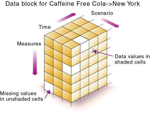
A data block is created for each unique combination of members in the Product and Market dimensions (see Data Storage). Each data block represents data from the dense dimensions. The data blocks likely will have few empty cells.
For example, consider the sparse member combination Caffeine Free Cola (100-30), New York, in Figure 2-5:
-
If accounts data (represented by the Measures dimension) exists for this combination for January, it probably exists for February and for all members in the Year dimension.
-
If a data value exists for one member on the Measures dimension, it is likely that other accounts data values exist for other members in the Measures dimension.
-
If Actual accounts data values exist, it is likely that Budget accounts data values exist.
Figure 2-5 Dense Data Block for Sample.Basic Database
Dense and Sparse Selection Scenarios
In the following scenarios, you'll see how a database is affected when you select different standard dimensions. Assume that these scenarios are based on typical databases with at least seven dimensions and several hundred members.
Scenario 1: All Sparse Standard Dimensions
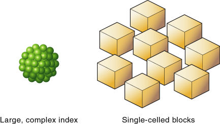
If you make all dimensions sparse, Essbase creates data blocks that consist of single data cells that contain single data values. An index entry is created for each data block and, therefore, in this scenario, for each existing data value.
This configuration produces an index that requires a large memory. The more index entries, the longer Essbase searches for a specific block.
Figure 2-6 Database with All Sparse Standard Dimensions
Scenario 2: All Dense Standard Dimensions
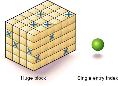
If you make all dimensions dense, Essbase creates one index entry and one large, sparse block. In most applications, this configuration requires thousands of times more storage than other configurations. Essbase must load the entire database into memory when it searches for any data value, which requires enormous memory.
Figure 2-7 Database with All Dense Standard Dimensions
Scenario 3: Dense and Sparse Standard Dimensions
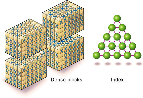
Based on your knowledge of your company’s data, you have identified all your sparse and dense standard dimensions.
Essbase creates dense blocks that can fit into memory easily and creates a relatively small index. Your database runs efficiently using minimal resources.
Figure 2-8 An Ideal Configuration with Combination of Dense and Sparse Dimensions
Scenario 4: A Typical Multidimensional Problem
Consider a database with four standard dimensions: Time, Accounts, Region, and Product. In the following example, Time and Accounts are dense dimensions, and Region and Product are sparse dimensions.
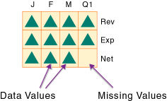
The two-dimensional data blocks shown in the image below represent data values from the dense dimensions: Time and Accounts. The members in the Time dimension are J, F, M, and Q1. The members in the Accounts dimension are Rev, Exp, and Net.
Figure 2-9 Two-dimensional Data Block for Time and Accounts
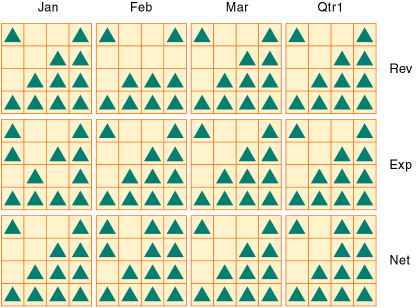
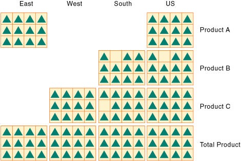
Essbase creates data blocks for combinations of members in the sparse standard dimensions (providing that at least one data value exists for the member combination). The sparse dimensions are Region and Product. The members of the Region dimension are East, West, South, and Total US. The members in the Product dimension are Product A, Product B, Product C, and Total Product.
The image below shows 11 data blocks. No data values exist for Product A in the West and South, for Product B in the East and West, or for Product C in the East. Therefore, Essbase has not created data blocks for these member combinations. The data blocks that Essbase has created have few empty cells. This example effectively concentrates all sparseness into the index and concentrates all data into fully utilized blocks. This configuration provides efficient data storage and retrieval.
Figure 2-10 Data Blocks Created for Sparse Members on Region and Product
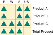
Next, consider a reversal of the dense and sparse dimension selections. In the following example, Region and Product are dense dimensions, and Time and Accounts are sparse dimensions.
In the image below, the two-dimensional data blocks represent data values from the dense dimensions: Region and Product. In the West region, data is not available for Product A and Product B. Data is also not available for Total Product in US.
Figure 2-11 Two-Dimensional Data Block for Region and Product
Essbase creates data blocks for combinations of members in the sparse standard dimensions (providing that at least one data value exists for the member combination). The sparse standard dimensions are Time and Accounts.
The image below shows 12 data blocks. Data values exist for all combinations of members in the Time and Accounts dimensions; therefore, Essbase creates data blocks for all member combinations. Because data values do not exist for all products in all regions, the data blocks have many empty cells. Data blocks with many empty cells store data inefficiently.
Figure 2-12 Data Blocks Created for Sparse Members on Time and Accounts
