8 Creating and Using Mappings
This chapter describes how to create and use mappings.
This chapter includes the following sections:
Introduction to Mappings
Mappings are the logical and physical organization of your data sources, targets, and the transformations through which the data flows from source to target. You create and manage mappings using the mapping editor, a new feature of ODI 12c.
The mapping editor opens whenever you open a mapping. Mappings are organized in folders under individual projects, found under Projects in the Designer Navigator.
Parts of a Mapping
A mapping is made up of and defined by the following parts:
-
Datastores
Data from source datastores is extracted by a mapping, and can be filtered during the loading process. Target datastores are the elements that are loaded by the mapping. Datastores act as Projector Components.
Datastores that will be used as sources and targets of the loading process must exist in data models before you can use them in a mapping. See Chapter 3, "Creating and Using Data Models and Datastores" for more information.
-
Datasets
Optionally, you can use datasets within mappings as sources. A Dataset is a logical container organizing datastores by an entity relationship declared as joins and filters, rather than the flow mechanism used elsewhere in mappings. Datasets operate similarly to ODI 11g interfaces, and if you import 11g interfaces into ODI 12c, ODI will automatically create datasets based on your interface logic. Datasets act as Selector Components.
-
Reusable Mappings
Reusable mappings are modular, encapsulated flows of components which you can save and re-use. You can place a reusable mapping inside another mapping, or another reusable mapping (that is, reusable mappings may be nested). A reusable mapping can also include datastores as sources and targets itself, like other mapping components. Reusable mappings act as Projector Components.
-
Other Components
ODI provides additional components that are used in between sources and targets to manipulate the data. These components are available on the component palette in the mapping diagram.
The following are the components available by default in the component palette:
-
Expression
-
Aggregate
-
Distinct
-
Set
-
Filter
-
Join
-
Lookup
-
Pivot
-
Sort
-
Split
-
Subquery Filter
-
Table Function
-
Unpivot
-
-
Connectors
Connectors create a flow of data between mapping components. Most components can have both input and output connectors. Datastores with only output connectors are considered sources; datastores with only input connectors are considered targets. Some components can support multiple input or output connectors; for example, the split component supports two or more output connectors, allowing you to split data into multiple downstream flows.
-
Connector points define the connections between components inside a mapping. A connector point is a single pathway for input or output for a component.
-
Connector ports are the small circles on the left and/or right sides of components displayed in the mapping diagram.
In the mapping diagram, two components connected by a single visible line between their connector ports could have one or more connector points. The diagram only shows a single line to represent all of the connections between two components. You can select the line to show details about the connection in the property inspector.
-
-
Staging Schemas
Optionally, you can specify a staging area for a mapping or for a specific physical mapping design of a mapping. If you want to define a different staging area than any of the source or target datastores, you must define the correct physical and logical schemas in the mapping's execution context before creating a mapping. See Chapter 2, "Overview of Oracle Data Integrator Topology" for more information.
-
Knowledge Modules
Knowledge modules define how data will be transferred between data servers and loaded into data targets. Knowledge Modules (IKMs, LKMs, EKMs, and CKMs) that will be selected in the flow must be imported into the project or must be available as global Knowledge Modules.
IKMs allow you to define (or specify) how the actual transformation and loading is performed.
LKMs allow you to specify how the transfer of the data between one data server to another data server is performed.
When used as flow control, CKMs allow you to check for errors in the data flow during the loading of records into a target datastore. When used as static control, CKMs can be used to check for any errors in a table. You can launch static control at any time on a model to see if the data satisfies constraints.
You can select a strategy to perform these tasks by selecting an appropriate KM. For example, you can decide whether to use a JDBC to transfer data between two databases, or use an Oracle database link if the transfer is between two Oracle databases.
See Chapter 6, "Creating an Integration Project" for more information.
-
Variables, Sequences, and User Functions
Variables, Sequences, and User Functions that will be used in expressions within your mappings must be created in the project. See Chapter 10, "Creating and Using Procedures, Variables, Sequences, and User Functions" for more information.
Navigating the Mapping Editor
The mapping editor provides a single environment for designing and editing mappings.
Mappings are organized within folders in a project in the Designer Navigator. Each folder has a mappings node, within which all mappings are listed.
To open the mapping editor, right-click an existing mapping and select Open, or double-click the mapping. To create a new mapping, right-click the Mappings node and select New Mapping. The mapping is opened as a tab on the main pane of ODI Studio. Select the tab corresponding to a mapping to view the mapping editor.
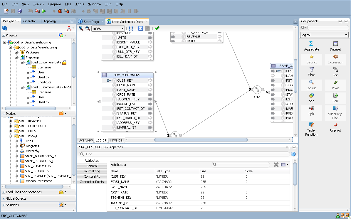
The mapping editor consists of the sections described in Table 8-1:
Table 8-1 Mapping Editor Sections
| Section | Location in Figure 8-1 | Description |
|---|---|---|
|
Mapping Diagram |
Middle |
The mapping diagram displays an editable logical or physical view of a mapping. These views are sometimes called the logical diagram or the physical diagram. You can drag datastores into the diagram from the Models tree, and Reusable Mappings from the Global Objects or Projects tree, into the mapping diagram. You can also drag components from the component palette to define various data operations. |
|
Mapping Editor tabs |
Middle, at the bottom of the mapping diagram |
The Mapping Editor tabs are ordered according to the mapping creation process. These tabs are:
|
|
Property Inspector |
Bottom |
Displays properties for the selected object. If the Property Inspector does not display, select Properties from the Window menu. |
|
Component Palette |
Right |
Displays the mapping components you can use for creating mappings. You can drag and drop components into the logical mapping diagram from the components palette. If the Component Palette does not display, select Components from the Window menu. |
|
Structure Panel |
Not shown |
Displays a text-based hierarchical tree view of a mapping, which is navigable using the tab and arrow keys. The Structure Panel does not display by default. To open it, select Structure from the Window menu. |
|
Thumbnail Panel |
Not shown |
Displays a miniature graphic of a mapping, with a rectangle indicating the portion currently showing in the mapping diagram. This panel is useful for navigating very large or complex mappings. The Thumbnail Panel does not display by default. To open it, select Thumbnail from the Window menu. |
Creating a Mapping
Creating a mapping follows a standard process which can vary depending on the use case.
Using the logical diagram of the mapping editor, you can construct your mapping by dragging components onto the diagram, dragging connections between the components, dragging attributes across those connections, and modifying the properties of the components using the property inspector. When the logical diagram is complete, you can use the physical diagram to define where and how the integration process will run on your physical infrastructure. When the logical and physical design of your mapping is complete, you can run it.
The following step sequence is usually performed when creating a mapping, and can be used as a guideline to design your first mappings:
Note:
You can also use the Property Inspector and the Structure Panel to perform the steps 2 to 5. See "Editing Mappings Using the Property Inspector and the Structure Panel" for more information.Creating a New Mapping
To create a new mapping:
-
In Designer Navigator select the Mappings node in the folder under the project where you want to create the mapping.
-
Right-click and select New Mapping. The New Mapping dialog is displayed.
-
In the New Mapping dialog, fill in the mapping Name. Optionally, enter a Description. If you want the new mapping to contain a new empty dataset, select Create Empty Dataset. Click OK.
Note:
You can add and remove datasets (including this empty dataset) after you create a mapping. Datasets are entirely optional and all behavior of a dataset can be created using other components in the mapping editor.In ODI 12c, Datasets offer you the option to create data flows using the entity relationship method familiar to users of previous versions of ODI. In some cases creating an entity relationship diagram may be faster than creating a flow diagram, or make it easier and faster to introduce changes.
When a physical diagram is calculated based on a logical diagram containing a Dataset, the entity relationships in the Dataset are automatically converted by ODI into a flow diagram and merged with the surrounding flow. You do not need to be concerned with how the flow is connected.
Your new mapping opens in a new tab in the main pane of ODI Studio.
Tip:
To display the editor of a datastore, a reusable mapping, or a dataset that is used in the Mapping tab, you can right-click the object and select Open.
Adding and Removing Components
Add components to the logical diagram by dragging them from the Component Palette. Drag datastores and reusable mappings from the Designer Navigator.
Delete components from a mapping by selecting them, and then either pressing the Delete key, or using the right-click context menu to select Delete. A confirmation dialog is shown.
Source and target datastores are the elements that will be extracted by, and loaded by, the mapping.
Between the source and target datastores are arranged all the other components of a mapping. When the mapping is run, data will flow from the source datastores, through the components you define, and into the target datastores.
Preserving and Removing Downstream Expressions
Where applicable, when you delete a component, a check box in the confirmation dialog allows you to preserve, or remove, downstream expressions; such expressions may have been created when you connected or modified a component. By default ODI preserves these expressions.
This feature allows you to make changes to a mapping without destroying work you have already done. For example, when a source datastore is mapped to a target datastore, the attributes are all mapped. You then realize that you need to filter the source data. To add the filter, one option is to delete the connection between the two datastores, but preserve the expressions set on the target datastore, and then connect a filter in the middle. None of the mapping expressions are lost.
Connecting and Configuring Components
Create connectors between components by dragging from the originating connector port to the destination connector port. Connectors can also be implicitly created by dragging attributes between components. When creating a connector between two ports, an attribute matching dialog may be shown which allows you to automatically map attributes based on name or position.
Attribute Matching
The Attribute Matching Dialog is displayed when a connector is drawn to a projector component (see: "Projector Components") in the Mapping Editor. The Attribute Matching Dialog gives you an option to automatically create expressions to map attributes from the source to the target component based on a matching mechanism. It also gives the option to create new attributes on the target based on the source, or new attributes on the source based on the target.
This feature allows you to easily define a set of attributes in a component that are derived from another component. For example, you could drag a connection from a new, empty Set component to a downstream target datastore. If you leave checked the Create Attributes On Source option in the Attribute Matching dialog, the Set component will be populated with all of the attributes of the target datastore. When you connect the Set component to upstream components, you will already have the target attributes ready for you to map the upstream attributes to.
Connector Points and Connector Ports
Review "Connectors" for an introduction to ODI connector terminology.
You can click a connector port on one component and drag a line to another component's connector port to define a connection. If the connection is allowed, ODI will either use an unused existing connector point on each component, or create an additional connector point as needed. The connection is displayed in the mapping diagram with a line drawn between the connector ports of the two connected components. Only a single line is shown even if two components have multiple connections between them.
Most components can use both input and output connectors to other components, which are visible in the mapping diagram as small circles on the sides of the component. The component type may place limitations on how many connectors of each type are allowed, and some components can have only input or only output connections.
Some components allow the addition or deletion of connector points using the property inspector.
For example, a Join component by default has two input connector points and one output connector point. It is allowed to have more than two inputs, though. If you drag a third connection to the input connector port of a join component, ODI creates a third input connector point. You can also select a Join component and, in the property inspector, in the Connector Points section, click the green plus icon to add additional Input Connector Points.
Note:
You cannot drag a connection to or from an input port that already has the maximum number of connections. For example, a target datastore can only have one input connector point; if you try to drag another connection to the input connector port, no connection is created.You can delete a connector by right-clicking the line between two connector points and selecting Delete, or by selecting the line and pressing the Delete key.
Defining New Attributes
When you add components to a mapping, you may need to create attributes in them in order to move data across the flow from sources, through intermediate components, to targets. Typically you define new attributes to perform transformations of the data.
Use any of the following methods to define new attributes:
-
Attribute Matching Dialog: This dialog is displayed in certain cases when dragging a connection from a connector port on one component to a connector port on another, when at least one component is a projector component.
The attribute matching dialog includes an option to create attributes on the target. If target already has attributes with matching names, ODI will automatically map to these attributes. If you choose By Position, ODI will map the first attributes to existing attributes in the target, and then add the rest (if there are more) below it. For example, if there are three attributes in the target component, and the source has 12, the first three attributes map to the existing attributes, and then the remaining nine are copied over with their existing labels.
-
Drag and drop attributes: Drag and drop a single (or multi-selected) attribute from a one component into another component (into a blank area of the component graphic, not on top of an existing attribute). ODI creates a connection (if one did not already exist), and also creates the attribute.
Tip:
If the graphic for a component is "full", you can hover over the attributes and a scroll bar appears on the right. Scroll to the bottom to expose a blank line. You can then drag attributes to the blank area.If you drag an attribute onto another attribute, ODI maps it into that attribute, even if the names do not match. This does not create a new attribute on the target component.
-
Add new attributes in the property inspector: In the property inspector, on the Attributes tab, use the green plus icon to create a new attribute. You can select or enter the new attribute's name, data type, and other properties in the Attributes table. You can then map to the new attribute by dragging attributes from other components onto the new attribute.
Caution:
ODI will allow you to create an illegal data type connection. Therefore, you should always set the appropriate data type when you create a new attribute. For example, if you intend to map an attribute with a DATE data type to a new attribute, you should set the new attribute to have the DATE type as well.Type-mismatch errors will be caught during execution as a SQL error.
Defining Expressions and Conditions
Expressions and conditions are used to map individual attributes from component to component. Component types determine the default expressions and conditions that will be converted into the underlying code of your mapping.
For example, any target component has an expression for each attribute. A filter, join, or lookup component will use code (such as SQL) to create the expression appropriate to the component type.
Tip:
When an expression is set on the target, any source attributes referenced by that expression are highlighted in magenta in the upstream sources. For example, an expressionemp.empno on the target column tgt_empno, when tgt_empno is selected (by clicking on it), the attribute empno on the source datastore emp is highlighted.
This highlighting function is useful for rapidly verifying that each desired target attribute has an expression with valid cross references. If an expression is manually edited incorrectly, such as if a source attribute is misspelled, the cross reference will be invalid, and no source attribute will be highlighted when clicking that target attribute.
You can modify the expressions and conditions of any component by modifying the code displayed in various property fields.
Note:
Oracle recommends using the expression editor instead of manually editing expressions in most cases. Selection of a source attribute from the expression editor will always give the expression a valid cross reference, minimizing editing errors. For more information, see "The Expression Editor".Expressions have a result type, such as VARCHAR or NUMERIC. The result type of conditions are boolean, meaning, the result of a condition should always evaluate to TRUE or FALSE. A condition is needed for filter, join, and lookup (selector) components, while an expression is used in datastore, aggregate, and distinct (projector) components, to perform some transformation or create the attribute-level mappings.
Every projector component can have expressions on its attributes. (For most projector components, an attribute has one expression, but the attribute of the Set component can have multiple expressions.) If you modify the expression for an attribute, a small "f" icon appears on the attribute in the logical diagram. This icon provides a visual cue that a function has been placed there.
To define the mapping of a target attribute:
-
In the mapping editor, select an attribute to display the attribute's properties in the Property Inspector.
-
In the Target tab (for expressions) or Condition tab (for conditions), modify the Expression or Condition field(s) to create the required logic.
Tip:
The attributes from any component in the diagram can be drag-and-dropped into an expression field to automatically add the fully-qualified attribute name to the code. -
Optionally, select or hover over any field in the property inspector containing an expression, and then click the gear icon that appears to the right of the field, to open the advanced Expression Editor.
The attributes on the left are only the ones that are in scope (have already been connected). So if you create a component with no upstream or downstream connection to a component with attributes, no attributes are listed.
-
Optionally, after modifying an expression or condition, consider validating your mapping to check for errors in your SQL code. Click the green check mark icon at the top of the logical diagram. Validation errors, if any, will be displayed in a panel.
Defining a Physical Configuration
In the Physical tab of the mapping editor, you define the loading and integration strategies for mapped data. Oracle Data Integrator automatically computes the flow depending on the configuration in the mapping's logical diagram. It proposes default knowledge modules (KMs) for the data flow. The Physical tab enables you to view the data flow and select the KMs used to load and integrate data.
For more information about physical design, see "Physical Design".
Running Mappings
Once a mapping is created, you can run it. This section briefly summarizes the process of running a mapping. For detailed information about running your integration processes, see: "Running Integration Processes" in Administering Oracle Data Integrator.
To run a mapping:
-
From the Projects menu of the Designer Navigator, right-click a mapping and select Run.
Or, with the mapping open in the mapping editor, click the run icon in the toolbar. Or, select Run from the Run menu.
-
In the Run dialog, select the execution parameters:
-
Select the Context into which the mapping must be executed. For more information about contexts, see: "Contexts".
-
Select the Physical Mapping Design you want to run. See: "Creating and Managing Physical Mapping Designs".
-
Select the Logical Agent that will run the mapping. The object can also be executed using the agent that is built into Oracle Data Integrator Studio, by selecting Local (No Agent). For more information about logical agents, see: "Agents".
-
Select a Log Level to control the detail of messages that will appear in the validator when the mapping is run. For more information about logging, see: "Managing the Log" in Administering Oracle Data Integrator.
-
Check the Simulation box if you want to preview the code without actually running it. In this case no data will be changed on the source or target datastores. For more information, see: "Simulating an Execution" in Administering Oracle Data Integrator.
-
-
Click OK.
-
The Information dialog appears. If your session started successfully, you will see "Session started."
-
Click OK.
Notes:
-
When you run a mapping, the Validation Results pane opens. You can review any validation warnings or errors there.
-
You can see your session in the Operator navigator Session List. Expand the Sessions node and then expand the mapping you ran to see your session. The session icon indicates whether the session is still running, completed, or stopped due to errors. For more information about monitoring your sessions, see: "Monitoring Integration Processes" in Administering Oracle Data Integrator.
-
Using Mapping Components
In the logical view of the mapping editor, you design a mapping by combining datastores with other components. You can use the mapping diagram to arrange and connect components such as datasets, filters, sorts, and so on. You can form connections between datastores and components by dragging lines between the connector ports displayed on these objects.
Mapping components can be divided into two categories which describe how they are used in a mapping: projector components and selector components.
Projectors are components that influence the attributes present in the data that flows through a mapping. Projector components define their own attributes: attributes from preceding components are mapped through expressions to the projector's attributes. A projector hides attributes originating from preceding components; all succeeding components can only use the attributes from the projector.
Review the following topics to learn how to use the various projector components:
Selector components reuse attributes from preceding components. Join and Lookup selectors combine attributes from the preceding components. For example, a Filter component following a datastore component reuses all attributes from the datastore component. As a consequence, selector components don't display their own attributes in the diagram and as part of the properties; they are displayed as a round shape. (The Expression component is an exception to this rule.)
When mapping attributes from a selector component to another component in the mapping, you can select and then drag an attribute from the source, across a chain of connected selector components, to a target datastore or next projector component. ODI will automatically create the necessary queries to bring that attribute across the intermediary selector components.
Review the following topics to learn how to use the various selector components:
The Expression Editor
Most of the components you use in a mapping are actually representations of an expression in the code that acts on the data as it flows from your source to your target datastores. When you create or modify these components, you can edit the expression's code directly in the Property Inspector.
To assist you with more complex expressions, you can also open an advanced editor called the Expression Editor. (In some cases, the editor is labeled according to the type of component; for example, from a Filter component, the editor is called the Filter Condition Advanced Editor. However, the functionality provided is the same.)
To access the Expression Editor, select a component, and in the Property Inspector, select or hover over with the mouse pointer any field containing code. A gear icon appears to the right of the field. Click the gear icon to open the Expression Editor.
For example, to see the gear icon in a Filter component, select or hover over the Filter Condition field on the Condition tab; to see the gear icon in a Datastore component, select or hover over the Journalized Data Filter field of the Journalizing tab.
A typical example view of the Expression Editor is shown in Figure 8-2
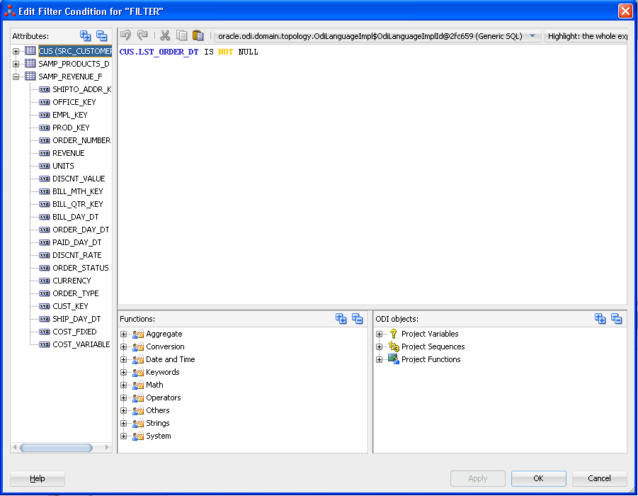
The Expression Editor is made up of the following panels:
-
Attributes: This panel appears on the left of the Expression Editor. When editing an expression for a mapping, this panel contains the names of attributes which are "in scope," meaning, attributes that are currently visible and can be referenced by the expression of the component. For example, if a component is connected to a source datastore, all of the attributes of that datastore are listed.
-
Expression: This panel appears in the middle of the Expression Editor. It displays the current code of the expression. You can directly type code here, or drag and drop elements from the other panels.
-
Technology functions: This panel appears below the expression. It lists the language elements and functions appropriate for the given technology.
-
Variables, Sequences, User Functions and odiRef API: This panel appears to the right of the technology functions and contains:
-
Project and global Variables.
-
Project and global Sequences.
-
Project and global User-Defined Functions.
-
OdiRef Substitution Methods.
-
Standard editing functions (cut/copy/paste/undo/redo) are available using the tool bar buttons.
Source and Target Datastores
To insert a source or target datastore in a mapping:
-
In the Designer Navigator, expand the Models tree and expand the model or sub-model containing the datastore to be inserted as a source or target.
-
Select this datastore, then drag it into the mapping panel. The datastore appears.
-
To make the datastore a source, drag a link from the output (right) connector of the datastore to one or more components. A datastore is not a source until it has at least one outgoing connection.
To make the datastore a target, drag a link from a component to the input (left) connector of the datastore. A datastore is not a target until it has an incoming connection.
Once you have defined a datastore you may wish to view its data.
To display the data of a datastore in a mapping:
-
Right-click the title of the datastore in the mapping diagram.
-
Select Data...
The Data Editor opens.
Creating Multiple Targets
In Oracle Data Integrator 12c, creating multiple targets in a mapping is straightforward. Every datastore component which has inputs but no outputs in the logical diagram is considered a target.
ODI allows splitting a component output into multiple flows at any point of a mapping. You can also create a single mapping with multiple independent flows, avoiding the need for a package to coordinate multiple mappings.
The output port of many components can be connected to multiple downstream components, which will cause all rows of the component result to be processed in each of the downstream flows. If rows should be routed or conditionally processed in the downstream flows, consider using a split component to define the split conditions.
See Also:
"Creating Splits"Specifying Target Order
Mappings with multiple targets do not, by default, follow a defined order of loading data to targets. You can define a partial or complete order by using the Target Load Order property. Targets which you do not explicitly assign an order will be loaded in an arbitrary order by ODI.
Note:
Target load order also applies to reusable mappings. If a reusable mapping contains a source or a target datastore, you can include the reusable mapping component in the target load order property of the parent mapping.The order of processing multiple targets can be set in the Target Load Order property of the mapping:
-
Click the background in the logical diagram to deselect objects in the mapping. The property inspector displays the properties for the mapping.
-
In the property inspector, accept the default target load order, or enter a new target load order, in the Target Load Order field.
Note:
A default load order is automatically computed based on primary key/foreign key relationships of the target datastores in the mapping. You can modify this default if needed, even if the resultant load order conflicts with the primary key/foreign key relationship. A warning will be displayed when you validate the mapping in this case.Select or hover over the Target Load Order field and click the gear icon to open the Target Load Order Dialog. This dialog displays all available datastores (and reusable mappings containing datastores) that can be targets, allowing you to move one or more to the Ordered Targets field. In the Ordered Targets field, use the icons on the right to rearrange the order of processing.
Tip:
Target Order is useful when a mapping has multiple targets and there are foreign key (FK) relationships between the targets. For example, suppose a mapping has two targets calledEMP and DEPT, and EMP.DEPTNO is a FK to DEPT.DEPTNO. If the source data contains information about the employee and the department, the information about the department (DEPT) must be loaded first before any rows about the employee can be loaded (EMP). To ensure this happens, the target load order should be set to DEPT, EMP.Adding a Reusable Mapping
Reusable mappings may be stored within folders in a project, or as global objects within the Global Objects tree, of the Designer Navigator.
To add a reusable mapping to a mapping:
-
To add a reusable mapping stored within the current project:
In the Designer Navigator, expand the Projects tree and expand the tree for the project you are working on. Expand the Reusable Mappings node to list all reusable mappings stored within this project.
To add a global reusable mapping:
In the Designer Navigator, expand the Global Objects tree, and expand the Reusable Mappings node to list all global reusable mappings.
-
Select a reusable mapping, and drag it into the mapping diagram. A reusable mapping component is added to the diagram as an interface to the underlying reusable mapping.
Creating Aggregates
The aggregate component is a projector component (see: "Projector Components") which groups and combines attributes using aggregate functions, such as average, count, maximum, sum, and so on. ODI will automatically select attributes without aggregation functions to be used as group-by attributes. You can override this by using the Is Group By and Manual Group By Clause properties.
To create an aggregate component:
-
Drag and drop the aggregate component from the component palette into the logical diagram.
-
Define the attributes of the aggregate if the attributes will be different from the source components. To do this, select the Attributes tab in the property inspector, and click the green plus icon to add attributes. Enter new attribute names in the Target column and assign them appropriate values.
If attributes in the aggregate component will be the same as those in a source component, use attribute matching (see Step 4).
-
Create a connection from a source component by dragging a line from the connector port of the source to the connector port of the aggregate component.
-
The Attribute Matching dialog will be shown. If attributes in the aggregate component will be the same as those in a source component, check the Create Attributes on Target box (see: "Attribute Matching").
-
If necessary, map all attributes from source to target that were not mapped though attribute matching, and create transformation expressions as necessary (see: "Defining Expressions and Conditions").
-
In the property inspector, the attributes are listed in a table on the Attributes tab. Specify aggregation functions for each attribute as needed. By default all attributes not mapped using aggregation functions (such as sum, count, avg, max, min, and so on) will be used as Group By.
You can modify an aggregation expression by clicking the attribute. For example, if you want to calculate average salary per department, you might have two attributes: the first attribute called
AVG_SAL, which you give the expressionAVG(EMP.SAL), while the second attribute calledDEPTNOhas no expression. If Is Group By is set toAuto,DEPTNOwill be automatically included in theGROUP BYclause of the generated code.You can override this default by changing the property Is Group By on a given attribute from
AutotoYesorNo, by double-clicking on the table cell and selecting the desired option from the drop down list.You can set a different
GROUP BYclause other than the default for the entire aggregate component. Select the General tab in the property inspector, and then set a Manual Group by Clause. For example, set the Manual Group by Clause toYEAR(customer.birthdate)to group by birthday year. -
Optionally, add a
HAVINGclause by setting the HAVING property of the aggregate component: for example,SUM(order.amount) > 1000.
Creating Distincts
A distinct is a projector component (see: "Projector Components") that projects a subset of attributes in the flow. The values of each row have to be unique; the behavior follows the rules of the SQL DISTINCT clause.
To select distinct rows from a source datastore:
-
Drag and drop a Distinct component from the component palette into the logical diagram.
-
Connect the preceding component to the Distinct component by dragging a line from the preceding component to the Distinct component.
The Attribute Mapping Dialog will appear: select Create Attributes On Target to create all of the attributes in the Distinct component. Alternatively, you can manually map attributes as desired using the Attributes tab in the property inspector.
-
The distinct component will now filter all rows that have all projected attributes matching.
Creating Expressions
An expression is a selector component (see: "Selector Components") that inherits attributes from a preceding component in the flow and adds additional reusable attributes. An expression can be used to define a number of reusable expressions within a single mapping. Attributes can be renamed and transformed from source attributes using SQL expressions. The behavior follows the rules of the SQL SELECT clause.
The best use of an expression component is in cases where intermediate transformations are used multiple times, such as when pre-calculating fields that are used in multiple targets.
If a transformation is used only once, consider performing the transformation in the target datastore or other component.
Tip:
If you want to reuse expressions across multiple mappings, consider using reusable mappings or user functions, depending on the complexity. See: "Reusable Mappings", and "Working with User Functions".To create an expression component:
-
Drag and drop an Expression component from the component palette into the logical diagram.
-
Connect a preceding component to the Expression component by dragging a line from the preceding component to the Expression component.
The Attribute Mapping Dialog will appear; select Create Attributes On Target to create all of the attributes in the Expression component.
In some cases you might want the expression component to match the attributes of a downstream component. In this case, connect the expression component with the downstream component first and select Create Attributes on Source to populate the Expression component with attributes from the target.
-
Add attributes to the expression component as desired using the Attributes tab in the property inspector. It might be useful to add attributes for pre-calculated fields that are used in multiple expressions in downstream components.
-
Edit the expressions of individual attributes as necessary (see: "Defining Expressions and Conditions").
Creating Filters
A filter is a selector component (see: "Selector Components") that can select a subset of data based on a filter condition. The behavior follows the rules of the SQL WHERE clause.
Filters can be located in a dataset or directly in a mapping as a flow component.
When used in a dataset, a filter is connected to one datastore or reusable mapping to filter all projections of this component out of the dataset. For more information, see Creating a Mapping Using a Dataset.
To define a filter in a mapping:
-
Drag and drop a Filter component from the component palette into the logical diagram.
-
Drag an attribute from the preceding component onto the filter component. A connector will be drawn from the preceding component to the filter, and the attribute will be referenced in the filter condition.
In the Condition tab of the Property Inspector, edit the Filter Condition and complete the expression. For example, if you want to select from the CUSTOMER table (that is the source datastore with the CUSTOMER alias) only those records with a NAME that is not null, an expression could be
CUSTOMER.NAME IS NOT NULL.Tip:
Click the gear icon to the right of the Filter Condition field to open the Filter Condition Advanced Editor. The gear icon is only shown when you have selected or are hovering over the Filter Condition field with your mouse pointer. For more information about the Filter Condition Advanced Editor, see: "The Expression Editor". -
Optionally, on the General tab of the Property Inspector, enter a new name in the Name field. Using a unique name is useful if you have multiple filters in your mapping.
-
Optionally, set an Execute on Hint, to indicate your preferred execution location:
No hint,Source,Staging, orTarget. The physical diagram will locate the execution of the filter according to your hint, if possible. For more information, see "Configuring Execution Locations".
Creating Joins and Lookups
This section contains the following topics:
A Join is a selector component (see: "Selector Components") that creates a join between multiple flows. The attributes from upstream components are combined as attributes of the Join component.
A Join can be located in a dataset or directly in a mapping as a flow component. A join combines data from two or more data flows, which may be datastores, datasets, reusable mappings, or combinations of various components.
When used in a dataset, a join combines the data of the datastores using the selected join type. For more information, see Creating a Mapping Using a Dataset.
A join used as a flow component can join two or more sources of attributes, such as datastores or other upstream components. A join condition can be formed by dragging attributes from two or more components successively onto a join component in the mapping diagram; by default the join condition will be an equi-join between the two attributes.
A Lookup is a selector component (see: "Selector Components") that returns data from a lookup flow being given a value from a driving flow. The attributes of both flows are combined, similarly to a join component.
Lookups can be located in a dataset or directly in a mapping as a flow component.
When used in a dataset, a Lookup is connected to two datastores or reusable mappings combining the data of the datastores using the selected join type. For more information, see Creating a Mapping Using a Dataset.
Lookups used as flow components (that is, not in a dataset) can join two flows. A lookup condition can be created by dragging an attribute from the driving flow and then the lookup flow onto the lookup component; the lookup condition will be an equi-join between the two attributes.
The Multiple Match Rows property defines which row from the lookup result must be selected as the lookup result if the lookup returns multiple results. Multiple rows are returned when the lookup condition specified matches multiple records.
You can select one of the following options to specify the action to perform when multiple rows are returned by the lookup operation:
-
Error: multiple rows will cause a mapping failure
This option indicates that when the lookup operation returns multiple rows, the mapping execution fails.
Note:
In ODI 12.1.3, the Deprecated - Error: multiple rows will cause a mapping failure option with theEXPRESSION_IN_SELECToption value is deprecated. It is included for backward compatibility with certain patched versions of ODI 12.1.2.This option is replaced with the
ERROR_WHEN_MULTIPLE_ROWoption of Error: multiple rows will cause a mapping failure. -
All Rows (number of result rows may differ from the number of input rows)
This option indicates that when the lookup operation returns multiple rows, all the rows should be returned as the lookup result.
Note:
In ODI 12.1.3, the Deprecated - All rows (number of result rows may differ from the number of input rows option with theLEFT_OUTERoption value is deprecated. It is included for backward compatibility with certain patched versions of ODI 12.1.2.This option is replaced with the
ALL_ROWSoption of All rows (number of result rows may differ from the number of input rows. -
Select any single row
This option indicates that when the lookup operation returns multiple rows, any one row from the returned rows must be selected as the lookup result.
-
Select first single row
This option indicates that when the lookup operation returns multiple rows, the first row from the returned rows must be selected as the lookup result.
-
Select nth single row
This option indicates that when the lookup operation returns multiple rows, the nth row from the result rows must be selected as the lookup result. When you select this option, the Nth Row Number field appears, where you can specify the value of n.
-
Select last single row
This option indicates that when the lookup operation returns multiple rows, the last row from the returned rows must be selected as the lookup result.
Use the Lookup Attributes Default Value & Order By table to specify how the result set that contains multiple rows should be ordered, and what the default value should be if no matches are found for the input attribute in the lookup flow through the lookup condition. Ensure that the attributes are listed in the same order (from top to bottom) in which you want the result set to be ordered. For example, to implement an ordering such as ORDER BY attr2, attr3, and then attr1, the attributes should be listed in the same order. You can use the arrow buttons to change the position of the attributes to specify the order.
The No-Match Rows property indicates the action to be performed when there are no rows that satisfy the lookup condition. You can select one of the following options to perform when no rows are returned by the lookup operation:
-
Return no row
This option does not return any row when no row in the lookup results satisfies the lookup condition.
-
Return a row with the following default values
This option returns a row that contains default values when no row in the lookup results satisfies the lookup condition. Use the Lookup Attributes Default Value & Order By: table below this option to specify the default values for each lookup attribute.
To create a join or a lookup between two upstream components:
-
Drag a join or lookup from the component palette into the logical diagram.
-
Drag the attributes participating in the join or lookup condition from the preceding components onto the join or lookup component. For example, if attribute
IDfrom source datastoreCUSTOMERand thenCUSTIDfrom source datastoreORDERare dragged onto a join, then the join conditionCUSTOMER.ID = ORDER.CUSTIDis created.Note:
When more than two attributes are dragged into a join or lookup, ODI compares and combines attributes with an AND operator. For example, if you dragged attributes from sources A and B into a Join component in the following order:A.FIRSTNAME B.FIRSTNAME A.LASTNAME B.LASTNAME
The following join condition would be created:
A.FIRSTNAME=B.FIRSTNAME AND A.LASTNAME=B.LASTNAME
You can continue with additional pairs of attributes in the same way.
You can edit the condition after it is created, as necessary.
-
In the Condition tab of the Property Inspector, edit the Join Condition or Lookup Condition and complete the expression.
Tip:
Click the gear icon to the right of the Join Condition or Lookup Condition field to open the Expression Editor. The gear icon is only shown when you have selected or are hovering over the condition field with your mouse pointer. For more information about the Expression Editor, see: "The Expression Editor". -
Optionally, set an Execute on Hint, to indicate your preferred execution location:
No hint,Source,Staging, orTarget. The physical diagram will locate the execution of the filter according to your hint, if possible. -
For a join:
Select the Join Type by checking the various boxes (Cross, Natural, Left Outer, Right Outer, Full Outer (by checking both left and right boxes), or (by leaving all boxes empty) Inner Join). The text describing which rows are retrieved by the join is updated.
For a lookup:
Select the Multiple Match Rows by selecting an option from the drop down list. The Technical Description field is updated with the SQL code representing the lookup, using fully-qualified attribute names.
If applicable, use the Lookup Attributes Default Value & Order By table to specify how a result set that contains multiple rows should be ordered.
Select a value for the No-Match Rows property to indicate the action to be performed when there are no rows that satisfy the lookup condition.
-
Optionally, for joins, if you want to use an ordered join syntax for this join, check the Generate ANSI Syntax box.
The Join Order box will be checked if you enable Generate ANSI Syntax, and the join will be automatically assigned an order number.
-
For joins inside of datasets, define the join order. Check the Join Order check box, and then in the User Defined field, enter an integer. A join component with a smaller join order number means that particular join will be processed first among other joins. The join order number determines how the joins are ordered in the
FROMclause. A smaller join order number means that the join will be performed earlier than other joins. This is important when there are outer joins in the dataset.For example: A mapping has two joins, JOIN1 and JOIN2. JOIN1 connects A and B, and its join type is
LEFT OUTER JOIN. JOIN2 connects B and C, and its join type isRIGHT OUTER JOIN.To generate
(A LEFT OUTER JOIN B) RIGHT OUTER JOIN C, assign a join order10for JOIN1 and20for JOIN2.To generate
A LEFT OUTER JOIN (B RIGHT OUTER JOIN C), assign a join order20forJOIN1and10for JOIN2.
Creating Pivots
A pivot component is a projector component (see: "Projector Components") that lets you transform data that is contained in multiple input rows into a single output row. The pivot component lets you extract data from a source once, and produce one row from a set of source rows that are grouped by attributes in the source data. The pivot component can be placed anywhere in the data flow of a mapping.
Example: Pivoting Sales Data
Table 8-2 shows a sample of data from the SALES relational table. The QUARTER attribute has 4 possible character values, one for each quarter of the year. All the sales figures are contained in one attribute, SALES.
| YEAR | QUARTER | SALES |
|---|---|---|
|
2010 |
Q1 |
10.5 |
|
2010 |
Q2 |
11.4 |
|
2010 |
Q3 |
9.5 |
|
2010 |
Q4 |
8.7 |
|
2011 |
Q1 |
9.5 |
|
2011 |
Q2 |
10.5 |
|
2011 |
Q3 |
10.3 |
|
2011 |
Q4 |
7.6 |
Table 8-3 depicts data from the relational table SALES after pivoting the table. The data that was formerly contained in the QUARTER attribute (Q1, Q2, Q3, and Q4) corresponds to 4 separate attributes (Q1_Sales, Q2_Sales, Q3_Sales, and Q4_Sales). The sales figures formerly contained in the SALES attribute are distributed across the 4 attributes for each quarter.
The Row Locator
When you use the pivot component, multiple input rows are transformed into a single row based on the row locator. The row locator is an attribute that you must select from the source to correspond with the set of output attributes that you define. It is necessary to specify a row locator to perform the pivot operation.
In this example, the row locator is the attribute QUARTER from the SALES table and it corresponds to the attributes Q1_Sales, Q2_Sales, Q3_Sales, and Q4_Sales attributes in the pivoted output data.
Using the Pivot Component
To use a pivot component in a mapping:
-
Drag and drop the source datastore into the logical diagram.
-
Drag and drop a Pivot component from the component palette into the logical diagram.
-
From the source datastore drag and drop the appropriate attributes on the pivot component. In this example, the YEAR attribute.
Note:
Do not drag the row locator attribute or the attributes that contain the data values that correspond to the output attributes. In this example, QUARTER is the row locator attribute and SALES is the attribute that contain the data values (sales figures) that correspond to the Q1_Sales, Q2_Sales, Q3_Sales, and Q4_Sales output attributes. -
Select the pivot component. The properties of the pivot component are displayed in the Property Inspector.
-
Enter a name and description for the pivot component.
-
If required, change the Aggregate Function for the pivot component. The default is
MIN. -
Type in the expression or use the Expression Editor to specify the row locator. In this example, since the QUARTER attribute in the SALES table is the row locator, the expression will be SALES.QUARTER.
-
Under Row Locator Values, click the + sign to add the row locator values. In this example, the possible values for the row locator attribute QUARTER are Q1, Q2, Q3, and Q4.
-
Under Attributes, add output attributes to correspond to each input row. If required, you can add new attributes or rename the listed attributes.
In this example, add 4 new attributes, Q1_Sales, Q2_Sales, Q3_Sales, and Q4_Sales that will correspond to 4 input rows Q1, Q2, Q3, and Q4 respectively.
-
If required, change the expression for each attribute to pick up the sales figures from the source and select a matching row for each attribute.
In this example, set the expressions for each attribute to SALES.SALES and set the matching rows to Q1, Q2, Q3, and Q4 respectively.
-
Drag and drop the target datastore into the logical diagram.
-
Connect the pivot component to the target datastore by dragging a link from the output (right) connector of the pivot component to the input (left) connector of the target datastore.
-
Drag and drop the appropriate attributes of the pivot component on to the target datastore. In this example, YEAR, Q1_Sales, Q2_Sales, Q3_Sales, and Q4_Sales.
-
Go to the physical diagram and assign new KMs if you want to.
Save and execute the mapping to perform the pivot operation.
Creating Sets
A set component is a projector component (see: "Projector Components") that combines multiple input flows into one using set operation such as UNION, INTERSECT, EXCEPT, MINUS and others. The behavior reflects the SQL operators.
Note:
PigSetCmd does not support the EXCEPT set operation.Additional input flows can be added to the set component by connecting new flows to it. The number of input flows is shown in the list of Input Connector Points in the Operators tab. If an input flow is removed, the input connector point needs to be removed as well.
To create a set from two or more sources:
-
Drag and drop a Set component from the component palette into the logical diagram.
-
Define the attributes of the set if the attributes will be different from the source components. To do this, select the Attributes tab in the property inspector, and click the green plus icon to add attributes. Select the new attribute names in the Target column and assign them appropriate values.
If Attributes will be the same as those in a source component, use attribute matching (see step 4).
-
Create a connection from the first source by dragging a line from the connector port of the source to the connector port of the Set component.
-
The Attribute Matching dialog will be shown. If attributes of the set should be the same as the source component, check the Create Attributes on Target box (see: "Attribute Matching").
-
If necessary, map all attributes from source to target that were not mapped through attribute matching, and create transformation expressions as necessary (see: "Defining Expressions and Conditions").
-
All mapped attributes will be marked by a yellow arrow in the logical diagram. This shows that not all sources have been mapped for this attribute; a set has at least two sources.
-
Repeat the connection and attribute mapping steps for all sources to be connected to this set component. After completion, no yellow arrows should remain.
-
In the property inspector, select the Operators tab and select cells in the Operator column to choose the appropriate set operators (
UNION,EXCEPT,INTERSECT, and so on).UNIONis chosen by default. You can also change the order of the connected sources to change the set behavior.
Note:
You can set Execute On Hint on the attributes of the set component, but there is also an Execute On Hint property for the set component itself. The hint on the component indicates the preferred location where the actual set operation (UNION, EXCEPT, and so on) is performed, while the hint on an attribute indicates where the preferred location of the expression is performed.
A common use case is that the set operation is performed on a staging execution unit, but some of its expressions can be done on the source execution unit. For more information about execution units, see "Configuring Execution Locations".
Creating Sorts
A Sort is a projector component (see: "Projector Components") that will apply a sort order to the rows of the processed dataset, using the SQL ORDER BY statement.
To create a sort on a source datastore:
-
Drag and drop a Sort component from the component palette into the logical diagram.
-
Drag the attribute to be sorted on from a preceding component onto the sort component. If the rows should be sorted based on multiple attributes, they can be dragged in desired order onto the sort component.
-
Select the sort component and select the Condition tab in the property inspector. The Sorter Condition field follows the syntax of the
SQL ORDER BYstatement of the underlying database; multiple fields can be listed separated by commas, andASCorDESCcan be appended after each field to define if the sort will be ascending or descending.
Creating Splits
A Split is a selector component (see: "Selector Components") that divides a flow into two or more flows based on specified conditions. Split conditions are not necessarily mutually exclusive: a source row is evaluated against all split conditions and may be valid for multiple output flows.
If a flow is divided unconditionally into multiple flows, no split component is necessary: you can connect multiple downstream components to a single outgoing connector port of any preceding component, and the data output by that preceding component will be routed to all downstream components.
A split component is used to conditionally route rows to multiple proceeding flows and targets.
To create a split to multiple targets in a mapping:
-
Drag and drop a Split component from the component palette into the logical diagram.
-
Connect the split component to the preceding component by dragging a line from the preceding component to the split component.
-
Connect the split component to each following component. If either of the upstream or downstream components contain attributes, the Attribute Mapping Dialog will appear. In the Connection Path section of the dialog, it will default to the first unmapped connector point and will add connector points as needed. Change this selection if a specific connector point should be used.
-
In the property inspector, open the Split Conditions tab. In the Output Connector Points table, enter expressions to select rows for each target. If an expression is left empty, all rows will be mapped to the selected target. Check the Remainder box to map all rows that have not been selected by any of the other targets.
Creating Subquery Filters
A subquery filter component is a projector component (see: "Projector Components") that lets you to filter rows based on the results of a subquery. The conditions that you can use to filter rows are EXISTS, NOT EXISTS, IN, and NOT IN.
For example, the EMP datastore contains employee data and the DEPT datastore contains department data. You can use a subquery to fetch a set of records from the DEPT datastore and then filter rows from the EMP datastore by using one of the subquery conditions.
A subquery filter component has two input connector points and one output connector point. The two input connector points are Driver Input connector point and Subquery Filter Input connector point. The Driver Input connector point is where the main datastore is set, which drives the whole query. The Subquery Filter Input connector point is where the datastore that is used in the sub-query is set. In the example, EMP is the Driver Input connector point and DEPT is the Subquery Filter Input connector point.
To filter rows using a subquery filter component:
-
Drag and drop a subquery filter component from the component palette into the logical diagram.
-
Connect the subquery filter component with the source datastores and the target datastore.
-
Drag and drop the input attributes from the source datastores on the subquery filter component.
-
Drag and drop the output attributes of the subquery filter component on the target datastore.
-
Go to the Connector Points tab and select the input datastores for the driver input connector point and the subquery filter input connector point.
-
Click the subquery filter component. The properties of the subquery filter component are displayed in the Property Inspector.
-
Go to the Attributes tab. The output connector point attributes are listed. Set the expressions for the driver input connector point and the subquery filter connector point.
Note:
You are required to set an expression for the subquery filter input connector point only if the subquery filter input role is set to one of the following:IN, NOT IN, =, >, <, >=, <=, !=, <>, ^=
-
Go to the Condition tab.
-
Type an expression in the Subquery Filter Condition field. It is necessary to specify a subquery filter condition if the subquery filter input role is set to EXISTS or NOT EXISTS.
-
Select a subquery filter input role from the Subquery Filter Input Role drop-down list.
-
Select a group comparison condition from the Group Comparison Condition drop-down list. A group comparison condition can be used only with the following subquery input roles:
=, >, <, >=, <=, !=, <>, ^=
-
Save and then execute the mapping.
Creating Table Functions
A table function component is a projector component (see: "Projector Components") that represents a table function in a mapping. Table function components enable you to manipulate a set of input rows and return another set of output rows of the same or different cardinality. The set of output rows can be queried like a physical table. A table function component can be placed anywhere in a mapping, as a source, a target, or a data flow component.
A table function component can have multiple input connector points and one output connector point. The input connector point attributes act as the input parameters for the table function, while the output connector point attributes are used to store the return values.
For each input connector, you can define the parameter type, REF_CURSOR or SCALAR, depending on the type of attributes the input connector point will hold.
To use a table function component in a mapping:
-
Create a table function in the database if it does not exist.
-
Right-click the Mappings node and select New Mapping.
-
Drag and drop the source datastore into the logical diagram.
-
Drag and drop a table function component from the component palette into the logical diagram. A table function component is created with no input connector points and one default output connector point.
-
Click the table function component. The properties of the table function component are displayed in the Property Inspector.
-
In the property inspector, go to the Attributes tab.
-
Type the name of the table function in the Name field. If the table function is in a different schema, type the function name as SCHEMA_NAME.FUNCTION_NAME.
-
Go to the Connector Points tab and click the + sign to add new input connector points. Do not forget to set the appropriate parameter type for each input connector.
Note:
Each REF_CURSOR attribute must be held by a separate input connector point with its parameter type set to REF_CURSOR. Multiple SCALAR attributes can be held by a single input connector point with its parameter type set to SCALAR. -
Go to the Attributes tab and add attributes for the input connector points (created in previous step) and the output connector point. The input connector point attributes act as the input parameters for the table function, while the output connector point attributes are used to store the return values.
-
Drag and drop the required attributes from the source datastore on the appropriate attributes for the input connector points of the table function component. A connection between the source datastore and the table function component is created.
-
Drag and drop the target datastore into the logical diagram.
-
Drag and drop the output attributes of the table function component on the attributes of the target datastore.
-
Go to the physical diagram of the mapping and ensure that the table function component is in the correct execution unit. If it is not, move the table function to the correct execution unit.
-
Assign new KMs if you want to.
-
Save and then execute the mapping.
Creating Unpivots
An unpivot component is a projector component (see: "Projector Components") that lets you transform data that is contained across attributes into multiple rows.
The unpivot component does the reverse of what the pivot component does. Similar to the pivot component, an unpivot component can be placed anywhere in the flow of a mapping.
The unpivot component is specifically useful in situations when you extract data from non-relational data sources such as a flat file, which contains data across attributes rather than rows.
Example: Unpivoting Sales Data
The external table, QUARTERLY_SALES_DATA, shown in Table 8-4, contains data from a flat file. There is a row for each year and separate attributes for sales in each quarter.
Table 8-4 QUARTERLY_SALES_DATA
| Year | Q1_Sales | Q2_Sales | Q3_Sales | Q4_Sales |
|---|---|---|---|---|
|
2010 |
10.5 |
11.4 |
9.5 |
8.7 |
|
2011 |
9.5 |
10.5 |
10.3 |
7.6 |
Table 8-5 shows a sample of the data after an unpivot operation is performed. The data that was formerly contained across multiple attributes (Q1_Sales, Q2_Sales, Q3_Sales, and Q4_Sales) is now contained in a single attribute (SALES). The unpivot component breaks the data in a single attribute (Q1_Sales) into two attributes (QUARTER and SALES). A single row in QUARTERLY_SALES_DATA corresponds to 4 rows (one for sales in each quarter) in the unpivoted data.
The Row Locator
The row locator is an output attribute that corresponds to the repeated set of data from the source. The unpivot component transforms a single input attribute into multiple rows and generates values for a row locator. The other attributes that correspond to the data from the source are referred as value locators. In this example, the attribute QUARTER is the row locator and the attribute SALES is the value locator.
Note:
To use the unpivot component, you are required to create the row locator and the value locator attributes for the unpivot component.The Value Locator field in the Unpivot Transforms table can be populated with an arbitrary expression. For example:
UNPIVOT_EMP_SALES.Q1_SALES + 100
Using the Unpivot Component
To use an unpivot component in a mapping:
-
Drag and drop the source data store into the logical diagram.
-
Drag and drop an unpivot component from the component palette into the logical diagram.
-
From the source datastore drag and drop the appropriate attributes on the unpivot component. In this example, the YEAR attribute.
Note:
Do not drag the attributes that contain the data that corresponds to the value locator. In this example, Q1_Sales, Q2_Sales, Q3_Sales, and Q4_Sales. -
Select the unpivot component. The properties of the unpivot component are displayed in the Property Inspector.
-
Enter a name and description for the unpivot component.
-
Create the row locator and value locator attributes using the Attribute Editor. In this example, you need to create two attributes named QUARTER and SALES.
Note:
Do not forget to define the appropriate data types and constraints (if required) for the attributes. -
In the Property Inspector, under UNPIVOT, select the row locator attribute from the Row Locator drop-down list. In this example, QUARTER.
Now that the row locator is selected, the other attributes can act as value locators. In this example, SALES.
-
Under UNPIVOT TRANSFORMS, click + to add transform rules for each output attribute. Edit the default values of the transform rules and specify the appropriate expressions to create the required logic.
In this example, you need to add 4 transform rules, one for each quarter. The transform rules define the values that will be populated in the row locator attribute QUARTER and the value locator attribute SALES. The QUARTER attribute must be populated with constant values (Q1, Q2, Q3, and Q4), while the SALES attribute must be populated with the values from source datastore attributes (Q1_Sales, Q2_Sales, Q3_Sales, and Q4_Sales).
-
Leave the INCLUDE NULLS check box selected to generate rows with no data for the attributes that are defined as NULL.
-
Drag and drop the target datastore into the logical diagram.
-
Connect the unpivot component to the target datastore by dragging a link from the output (right) connector of the unpivot component to the input (left) connector of the target datastore.
-
Drag and drop the appropriate attributes of the unpivot component on to the target datastore. In this example, YEAR, QUARTER, and SALES.
-
Go to the physical diagram and assign new KMs if you want to.
-
Click Save and then execute the mapping to perform the unpivot operation.
Creating Flatten Components
The flatten component is a Projector component that processes input data with complex structure and produces a flattened representation of the same data using standard datatypes.
The Flatten component has one input connector point and one output connector point.
To use a flatten component in a mapping:
-
Drag and drop the source data store into the logical diagram.
-
Drag and drop an flatten component from the component palette into the logical diagram.
-
Go to the physical diagram and assign new KMs if you want to.
-
Click Save and then execute the mapping to perform the flatten operation.
Creating Jagged Components
The jagged component is a Projector component that processes unstructured data using meta pivoting. With the jagged component, you can transform data into structured entities that can be loaded into database tables.
The jagged data component has one input group and multiple output groups, based on the configuration of the component.
The input group has two mandatory attributes: one each for name and value part of the incoming data set. A third, optional, attribute is used for row identifier sequences to delineate row sets.
To use a jagged component in a mapping:
-
Drag and drop the source data store into the logical diagram.
-
Drag and drop an jagged component from the component palette into the logical diagram.
-
The jagged input group requires two attribute level mappings; one for name and one for value.
-
Map one or more of the output groups to the downstream components.
Note:
In some cases, you may not need any additional attributes other than the default group: others. -
Go to the physical diagram and assign new KMs if you want to.
-
Click Save and then execute the mapping to perform the flatten operation.
Creating a Mapping Using a Dataset
A dataset component is a container component that allows you to group multiple data sources and join them through relationship joins. A dataset can contain the following components:
-
Datastores
-
Joins
-
Lookups
-
Filters
-
Reusable Mappings: Only reusable mappings with no input signature and one output signature are allowed.
Create Joins and lookups by dragging an attribute from one datastore to another inside the dataset. A dialog is shown to select if the relationship will be a join or lookup.
Note:
A driving table will have the key to look up, while the lookup table has additional information to add to the result.In a dataset, drag an attribute from the driving table to the lookup table. An arrow will point from the driving table to the lookup table in the diagram.
By comparison, in a flow-based lookup (a lookup in a mapping that is not inside a dataset), the driving and lookup sources are determined by the order in which connections are created. The first connection is called DRIVER_INPUT1, the second connection LOOKUP_INPUT1.
Create a filter by dragging a datastore or reusable mapping attribute onto the dataset background. Joins, lookups, and filters cannot be dragged from the component palette into the dataset.
This section contains the following topics:
Differences Between Flow and Dataset Modeling
Datasets are container components which contain one or more source datastores, which are related using filters and joins. To other components in a mapping, a dataset is indistinguishable from any other projector component (like a datastore); the results of filters and joins inside the dataset are represented on its output port.
Within a dataset, data sources are related using relationships instead of a flow. This is displayed using an entity relationship diagram. When you switch to the physical tab of the mapping editor, datasets disappear: ODI models the physical flow of data exactly the same as if a flow diagram had been defined in the logical tab of the mapping editor.
Datasets mimic the ODI 11g way of organizing data sources, as opposed to the flow metaphor used in an ODI 12c mapping. If you import projects from ODI 11g, interfaces converted into mappings will contain datasets containing your source datastores.
When you create a new, empty mapping, you are prompted whether you would like to include an empty dataset. You can delete this empty dataset without harm, and you can always add an empty dataset to any mapping. The option to include an empty dataset is purely for your convenience.
A dataset exists only within a mapping or reusable mapping, and cannot be independently designed as a separate object.
Creating a Dataset in a Mapping
To create a dataset in a mapping, drag a dataset from the component palette into the logical diagram. You can then drag datastores into the dataset from the Models section of the Designer Navigator. Drag attributes from one datastore to another within a dataset to define join and lookup relationships.
Drag a connection from the dataset's output connector point to the input connector point on other components in your mapping, to integrate it into your data flow.
See Also:
To create a Join or Lookup inside a Dataset, see: "Creating a Join or Lookup"Converting a Dataset to Flow-Based Mapping
You can individually convert datasets into a flow-based mapping diagram, which is merged with the parent mapping flow diagram.
The effect of conversion of a dataset into a flow is the permanent removal of the dataset, together with the entity relationship design. It is replaced by an equivalent flow-based design. The effect of the conversion is irreversible.
To convert a dataset into a flow-based mapping:
-
Select the dataset in the mapping diagram.
-
Right click on the title and select Convert to Flow from the context menu.
-
A warning and confirmation dialog is displayed. Click Yes to perform the conversion, or click No to cancel the conversion.
The dataset is converted into flow-based mapping components.
Physical Design
The physical tab shows the distribution of execution among different execution units that represent physical servers. ODI computes a default physical mapping design containing execution units and groups based on the logical design, the topology of those items and any rules you have defined.
You can also customize this design by using the physical diagram. You can use the diagram to move components between execution units, or onto the diagram background, which creates a separate execution unit. Multiple execution units can be grouped into execution groups, which enable parallel execution of the contained execution units.
A mapping can have multiple physical mapping designs; they are listed in tabs under the diagram. By having multiple physical mapping designs you can create different execution strategies for the same mapping.
To create new physical mapping tabs, click the Create New tab.
To delete physical mapping designs, right-click on the physical mapping design tab you want to delete, and select Delete from the context menu.
Physical components define how a mapping is executed at runtime; they are the physical representation of logical components. Depending on the logical component a physical component might have a different set of properties.
This section contains the following topics:
About the Physical Mapping Diagram
In the physical diagram, the following items appear:
-
Physical Mapping Design: The entire physical diagram represents one physical mapping design. Click the background or select the white tab with the physical mapping design label to display the physical mapping properties. By default, the staging location is colocated on the target, but you can explicitly select a different staging location to cause ODI to automatically move staging to a different host.
You can define additional physical mapping designs by clicking the small tab at the bottom of the physical diagram, next to the current physical mapping design tab. A new physical mapping design is created automatically from the logical design of the mapping.
-
Execution Groups: Yellow boxes display groups of objects called execution units, which are executed in parallel within the same execution group. These are usually Source Groups and Target Groups:
-
Source Execution Group(s): Source Datastores that are within the same dataset or are located on the same physical data server are grouped in a single source execution group in the physical diagram. A source execution group represents a group of datastores that can be extracted at the same time.
-
Target Execution Group(s): Target Datastores that are located on the same physical data server are grouped in a single target execution group in the physical diagram. A target execution group represents a group of datastores that can be written to at the same time.
-
-
Execution Units: Within the yellow execution groups are blue boxes called execution units. Execution units within a single execution group are on the same physical data server, but may be different structures.
-
Access Points: In the target execution group, whenever the flow of data goes from one execution unit to another there is an access point (shown with a round icon). Loading Knowledge Modules (LKMs) control how data is transferred from one execution unit to another.
An access point is created on the target side of a pair of execution units, when data moves from the source side to the target side (unless you use Execute On Hint in the logical diagram to suggest a different execution location). You cannot move an access point node to the source side. However, you can drag an access point node to the empty diagram area and a new execution unit will be created, between the original source and target execution units in the diagram.
-
Components: mapping components such as joins, filters, and so on are also shown on the physical diagram.
You use the following knowledge modules (KMs) in the physical tab:
-
Loading Knowledge Modules (LKMs): LKMs define how data is moved. One LKM is selected for each access point for moving data from the sources to a staging area. An LKM can be also selected to move data from a staging area not located within a target execution unit, to a target, when a single technology IKM is selected for the staging area. Select an access point to define or change its LKM in the property inspector.
-
Integration Knowledge Modules (IKMs) and Check Knowledge Modules (CKMs): IKMs and CKMs define how data is integrated into the target. One IKM and one CKM is typically selected on a target datastore. When the staging area is different from the target, the selected IKM can be a multi-technology IKM that moves and integrates data from the staging area into the target. Select a target datastore to define or change its IKM and CKM in the property inspector.
Notes:
-
Only built-in KMs, or KMs that have already been imported into the project or the global KM list, can be selected in the mapping. Make sure that you have imported the appropriate KMs in the project before proceeding.
-
For more information on the KMs and their options, refer to the KM description and to the Connectivity and Knowledge Modules Guide for Oracle Data Integrator.
Selecting LKMs, IKMs and CKMs
ODI automatically selects knowledge modules in the physical diagram as you create your logical diagram.
Note:
The Integration Type property of a target datastore (which can have the valuesControl Append, Incremental Update, or Slowly Changing Dimension) is referenced by ODI when it selects a KM. This property is also used to restrict the IKM selection shown, so you will only see IKMs listed that are applicable.You can use the physical diagram to change the KMs in use.
-
In the physical diagram, select an access point. The Property Inspector opens for this object.
-
Select the Loading Knowledge Module tab, and then select a different LKM from the Loading Knowledge Module list.
-
KMs are set with default options that work in most use cases. You can optionally modify the KM Options.
Note:
If an identically-named option exists, when switching from one KM to another KM options of the previous KM are retained. However, options that are not duplicated in the new KM are lost.
Note:
In order to use a multi-connect IKM on the target node, you must select LKM SQL Multi-Connect, or no LKM, for the access point of that execution unit. If another LKM is selected, only mono-connect IKMs are selectable.-
In the physical diagram, select a target datastore by clicking its title. The Property Inspector opens for this object.
-
In the Property Inspector, select the Integration Knowledge Module tab, and then select an IKM from the Integration Knowledge Module list.
-
KMs are set with default options that work in most use cases. You can optionally modify the KM Options.
Note:
If an identically-named option exists, when switching from one KM to another KM options of the previous KM are retained. However, options that are not duplicated in the new KM are lost.
-
In the physical diagram, select a target datastore by clicking its title. The Property Inspector opens for this object.
-
In the Property Inspector, select the Check Knowledge Module tab, and then select a CKM from the Check Knowledge Module list.
-
KMs are set with default options that work in most use cases. You can optionally modify the KM Options.
Note:
If an identically-named option exists, when switching from one KM to another KM options of the previous KM are retained. However, options that are not duplicated in the new KM are lost.
Configuring Execution Locations
In the physical tab of the mapping editor, you can change the staging area and determine where components will be executed. When you designed the mapping using components in the logical diagram, you optionally set preferred execution locations using the Execute On Hint property. In the physical diagram, ODI attempts to follow these hints where possible.
You can further manipulate execution locations in the physical tab. See the following topics for details:
Moving Physical Nodes
You can move the execution location of a physical node. Select the node and drag it from one Execution Group into another Execution Group. Or, drag it to a blank area of the physical diagram, and ODI will automatically create a new Execution Group for the component.
You can change the order of execution of certain components only. The following components can be reordered on the physical diagram:
-
Expressions
-
Filters
-
Joins
-
Lookups
Moving Expressions
You can move expressions in the physical diagram. Select the Execution Unit and in the property inspector, select the Expressions tab. The execution location of the expression is shown in the Execute on property. Double-click the property to alter the execution location.
Defining New Execution Units
You can define a new execution unit by dragging a component from its current execution unit onto a blank area of the physical diagram. A new execution unit and group is created. Select the execution unit to modify its properties using the property inspector.
Adding Commands to be Executed Before and After a Mapping
ODI allows the addition of commands to be executed before and after a mapping. These commands can be in ODI-supported languages such as SQL, Jython, Groovy, and others. In the SQL language the Begin Mapping and End Mapping commands are executed in the same transaction as the mapping. The physical design of a mapping has the following properties to control this behavior:
| Property | Description |
|---|---|
| Begin Mapping Command | Command to be executed at the beginning of the mapping. |
| Technology for Begin Mapping Command | Technology that this command will be executed with. |
| Location for Begin Mapping Command | Logical Schema that this command will be executed in. |
| End Mapping Command | Command to be executed at the end of the mapping. |
| Technology for End Mapping Command | Technology that this command will be executed with. |
| Location for End Mapping Command | Logical Schema that this command will be executed in. |
You can view and set these properties from the Property Inspector by selecting a Physical Mapping Design.
Configuring In-Session Parallelism
ODI agent is the scheduler that runs an entire ODI mapping job on a given host. If your have two or more loads, it will either run them one after another (serialized), or simultaneously (parallelized, using separate processor threads).
Execution units in the same execution group are parallelized. If you move an execution unit into its own group, it is no longer parallelized with other execution units: it is now serialized. The system will select the order in which separate execution groups are run.
You might choose to run loads serially to reduce instantaneous system resource usage, while you might choose to run loads in parallel to reduce the longevity of system resource usage.
Configuring Parallel Target Table Load
You can enable parallel target table loading in a physical mapping design. Select the physical mapping design (by clicking on the tab at the bottom of the physical diagram, or clicking an empty area of the diagram) and in the property inspector, check the box for the property Use Unique Temporary Object Names.
This option allows multiple instances of the same mapping to be executed concurrently. To load data from source to staging area, C$ tables are created in the staging database.
Note:
In ODI 11g,C$ table names were derived from the target table of the interface. As a result, when multiple instances of the same mapping were executed at the same time, data from different sessions could load into the same C$ table and cause conflicts.
In ODI 12c, if the option Use Unique Temporary Object Names is set to true, the system generates a globally-unique name for C$ tables for each mapping execution. This prevents any conflict from occurring.
Configuring Temporary Indexes
If you want ODI to automatically generate a temporary index to optimize the execution of a filter, join, or datastore, select the node in the physical diagram. In the property inspector, select the Temporary Indexes tab. You can double-click the Index Type field to select a temporary index type.
Note:
The creation of temporary indexes may be a time consuming operation in the overall flow. Oracle recommends reviewing execution statistics and comparing the execution time saved by the indexes to the time spent creating them.Configuring Journalizing
A source datastore can be configured in the physical diagram to use journalized data only. This is done by enabling Journalized Data Only in the General properties of a source datastore. The check box is only available if the referenced datastore is added to CDC in the model navigator.
Only one datastore per mapping can have journalizing enabled.
For more information about journalizing, see Chapter 4, "Using Journalizing."
Configuring Extraction Options
Each component in the physical diagram, excluding access points and target datastores, has an Extraction Options tab in the property inspector. Extraction options influence the way that SQL is generated for the given component. Most components have an empty list of extraction options, meaning that no further configuration of the SQL generation is supported.
Extraction options are driven by the Extract Knowledge Module (XKM) selected in the Advanced sub-tab of the Extract Options tab. XKMs are part of ODI and cannot be created or modified by the user.
Creating and Managing Physical Mapping Designs
The entire physical diagram represents one physical mapping design. Click the background or select the white tab with the physical mapping design label to display the physical mapping properties for the displayed physical mapping design.
You can define additional physical mapping designs by clicking the small tab at the bottom of the physical diagram, next to the current physical mapping design tab(s). A new physical mapping design is created automatically, generated from the logical design of the mapping. You can modify this physical mapping design, and save it as part of the mapping.
For example, you could use one physical mapping design for your initial load, and another physical mapping design for incremental load using changed data capture (CDC). The two physical mapping designs would have different journalizing and knowledge module settings.
As another example, you could use different optimization contexts for each physical mapping design. Each optimization context represents a slightly different users' topology. One optimization context can represent a development environment, and another context represents a testing environment. You could select different KMs appropriate for these two different topologies.
Reusable Mappings
Reusable mappings allow you to encapsulate a multi-step integration (or portion of an integration) into a single component, which you can save and use just as any other components in your mappings. Reusable mappings are a convenient way to avoid the labor of creating a similar or identical subroutine of data manipulation that you will use many times in your mappings.
For example, you could load data from two tables in a join component, pass it through a filter component, and then a distinct component, and then output to a target datastore. You could then save this procedure as a reusable mapping, and place it into future mappings that you create or modify.
After you place a reusable mapping component in a mapping, you can select it and make modifications to it that only affect the current mapping.
Reusable mappings consist of the following:
-
Input Signature and Output Signature components: These components describe the attributes that will be used to map into and out of the reusable mapping. When the reusable mapping is used in a mapping, these are the attributes that can be matched by other mapping components.
-
Regular mapping components: Reusable mappings can include all of the regular mapping components, including datastores, projector components, and selector components. You can use these exactly as in regular mappings, creating a logical flow.
By combining regular mapping components with signature components, you can create a reusable mapping intended to serve as a data source, as a data target, or as an intermediate step in a mapping flow. When you work on a regular mapping, you can use a reusable mapping as if it were a single component.
Creating a Reusable Mapping
You can create a reusable mapping within a project, or as a global object. To create a reusable mapping, perform the following steps:
-
From the designer navigator:
Open a project, right-click Reusable Mappings, and select New Reusable Mapping.
Or, expand the Global Objects tree, right click Global Reusable Mappings, and select New Reusable Mapping.
-
Enter a name and, optionally, a description for the new reusable mapping. Optionally, select Create Default Input Signature and/or Create Default Output Signature. These options add empty input and output signatures to your reusable mapping; you can add or remove input and output signatures later while editing your reusable mapping.
Note:
In order to make use of these signatures, you will need to connect them to your reusable mapping flow. -
Drag components from the component palette into the reusable mapping diagram, and drag datastores and other reusable mappings from the designer navigator, to assemble your reusable mapping logic. Follow all of the same processes as for creating a normal mapping.
Note:
When you have a reusable mapping open for editing, the component palette contains the Input Signature and Output Signature components in addition to the regular mapping components. -
Validate your reusable mapping by clicking the Validate the Mapping button (a green check mark icon). Any errors will be displayed in a new error pane.
When you are finished creating your reusable mapping, click File and select Save, or click the Save button, to save your reusable mapping. You can now use your reusable mapping in your mapping projects.
Editing Mappings Using the Property Inspector and the Structure Panel
You can use the Property Inspector with the Structure Panel to perform the same actions as on the logical and physical diagrams of the mapping editor, in a non-graphical form.
When creating and editing mappings without using the logical and physical diagrams, you will need to open the Structure Panel. The Structure Panel provides an expandable tree view of a mapping, which you can traverse using the tab keys, allowing you to select the components of your mapping. When you select a component or attribute in the Structure Panel, its properties are shown in the Property Inspector exactly the same as if you had selected the component in the logical or physical diagram.
The Structure Panel is useful for accessibility requirements, such as when using a screen reader.
To open the structure panel, select Window from the main menu and then click Structure. You can also open the Structure Panel using the hotkey Ctrl+Shift-S.
This section contains the following topics:
Adding and Removing Components
With the Property Inspector, the Component Palette, and the Structure Panel, you can add or remove components of a mapping.
Adding Components
To add a component to a mapping with the Component Palette and the Structure Panel:
-
With the mapping open in the Mapping Editor, open the Component Palette.
-
Select the desired component using the Tab key, and hit Enter to add the selected component to the mapping diagram and the Structure Panel.
Removing Components
To remove a component with the Structure Panel:
-
In the Structure Panel, select the component you want to remove.
-
While holding down Ctrl+Shift, hit Tab to open a pop-up dialog. Keep holding down Ctrl+Shift, and use the arrow keys to navigate to the left column and select the mapping. You can then use the right arrow key to select the logical or physical diagram. Release the Ctrl+Shift keys after you select the logical diagram.
Alternatively, select Windows > Documents... from the main menu bar. Select the mapping from the list of document windows, and click Switch to Document.
-
The component you selected in the Structure Panel in step 1 is now highlighted in the mapping diagram. Hit Delete to delete the component. A dialog box confirms the deletion.
Editing a Component
To edit a component of a mapping using the Structure Panel and the Property Inspector:
-
In the Structure Panel, select a component. The component's properties are shown in the Property Inspector.
-
In the Property Inspector, modify properties as needed. Use the Attributes tab to add or remove attributes. Use the Connector Points tab to add connections to other components in your mapping.
-
Expand any component in the Structure Panel to list individual attributes. You can then select individual attributes to show their properties in the Property Inspector.
Customizing Tables
There are two ways to customize the tables in the Property Inspector to affect which columns are shown. In each case, open the Structure Panel and select a component to display its properties in the Property Inspector. Then, select a tab containing a table and use one of the following methods:
-
From the table toolbar, click the Select Columns... icon (on the top right corner of the table) and then, from the drop down menu, select the columns to display in the table. Currently displayed columns are marked with a check mark.
-
Use the Customize Table Dialog:
-
From the table toolbar, click Select Columns....
-
From the drop down menu, select Select Columns...
-
In the Customize Table Dialog, select the columns to display in the table.
-
Click OK.
-
Using Keyboard Navigation for Common Tasks
This section describes the keyboard navigation in the Property Inspector.
Table 8-6 shows the common tasks and the keyboard navigation used in the Property Inspector.
Table 8-6 Keyboard Navigation for Common Tasks
| Navigation | Task |
|---|---|
|
Arrow keys |
Navigate: move one cell up, down, left, or right |
|
TAB |
Move to next cell |
|
SHIFT+TAB |
Move to previous cell |
|
SPACEBAR |
Start editing a text, display items of a list, or change value of a checkbox |
|
CTRL+C |
Copy the selection |
|
CTRL+V |
Paste the selection |
|
ESC |
Cancel an entry in the cell |
|
ENTER |
Complete a cell entry and move to the next cell or activate a button |
|
DELETE |
Clear the content of the selection (for text fields only) |
|
BACKSPACE |
Delete the content of the selection or delete the preceding character in the active cell (for text fields only) |
|
HOME |
Move to the first cell of the row |
|
END |
Move to the last cell of the row |
|
PAGE UP |
Move up to the first cell of the column |
|
PAGE DOWN |
Move down to the last cell of the column |
Flow Control and Static Control
In a mapping, it is possible to set two points of control. Flow Control checks the data in the incoming flow before it gets integrated into a target, and Static Control checks constraints on the target datastore after integration.
IKMs can have options to run FLOW_CONTROL and to run STATIC_CONTROL. If you want to enable either of these you must set the option in the IKM, which is a property set on the target datastore. In the physical diagram, select the datastore, and select the Integration Knowledge Module tab in the property inspector. If flow control options are available, they are listed in the Options table. Double-click an option to change it.
Notes:
-
Flow control is not supported for component KMs like IKM Oracle Insert. For more information, see "Knowledge Modules" in Connectivity and Knowledge Modules Guide for Oracle Data Integrator. The description of each IKM indicates if it supports flow control.
-
In ODI 11g the CKM to be used when flow or static control is invoked was defined on the interface. ODI 12c supports multiple targets on different technologies within the same mapping, so the CKM is now defined on each target datastore
This section contains the following topics:
Setting up Flow Control
The flow control strategy defines how data is checked against the constraints defined on a target datastore before being integrated into this datastore. It is defined by a Check Knowledge Module (CKM). The CKM can be selected on the target datastore physical node. The constraints that checked by a CKM are specified in the properties of the datastore component on the logical tab.
To define the CKM used in a mapping, see: "Selecting LKMs, IKMs and CKMs".
Setting up Static Control
The post-integration control strategy defines how data is checked against the constraints defined on the target datastore. This check takes place once the data is integrated into the target datastore. It is defined by a CKM. In order to have the post-integration control running, you must set the STATIC_CONTROL option in the IKM to true. Post-integration control requires that a primary key is defined in the data model for the target datastore of your mapping.
The settings Maximum Number of Errors Allowed and Integration Errors as Percentage can be set on the target datastore component. Select the datastore in the logical diagram, and in the property inspector, select the Target tab.
Post-integration control uses the same CKM as flow control.
Defining the Update Key
If you want to use update or flow control features in your mapping, it is necessary to define an update key on the target datastore.
The update key of a target datastore component contains one or more attributes. It can be the unique key of the datastore that it is bound to, or a group of attributes that are marked as the key attribute. The update key identifies each record to update or check before insertion into the target.
To define the update key from a unique key:
-
In the mapping diagram, select the header of a target datastore component. The component's properties will be displayed in the Property Inspector.
-
In the Target properties, select an Update Key from the drop down list.
Notes:
-
The Target properties are only shown for datastores which are the target of incoming data. If you do not see the Target properties, your datastore does not have an incoming connection defined.
-
Only unique keys defined in the model for this datastore appear in this list.
You can also define an update key from the attributes if:
-
You don't have a unique key on your datastore.
-
You want to specify the key regardless of already defined keys.
When you define an update key from the attributes, you select manually individual attributes to be part of the update key.
To define the update key from the attributes:
-
Unselect the update key, if it is selected.
-
In the Target Datastore panel, select one of the attributes that is part of the update key to display the Property Inspector.
-
In the Property Inspector, under Target properties, check the Key box. A key symbol appears in front of the key attribute(s) in the datastore component displayed in the mapping editor logical diagram.
-
Repeat the operation for each attribute that is part of the update key.
Designing E-LT and ETL-Style Mappings
See Also:
E-LT and ETL are defined and described in "What is E-LT" in Understanding Oracle Data Integrator.In an E-LT-style integration mapping, ODI processes the data in a staging area, which is located on the target. Staging area and target are located on the same RDBMS. The data is loaded from the source(s) to the target. To create an E-LT-style integration mapping, follow the standard procedure described in "Creating a Mapping".
In an ETL-style mapping, ODI processes the data in a staging area, which is different from the target. The data is first extracted from the source(s) and then loaded to the staging area. The data transformations take place in the staging area and the intermediate results are stored in temporary tables in the staging area. The data loading and transformation tasks are performed with the standard ELT KMs.
Oracle Data Integrator provides two ways for loading the data from the staging area to the target:
Depending on the KM strategy that is used, flow and static control are supported. See "Designing an ETL-Style Mapping" in the Connectivity and Knowledge Modules Guide for Oracle Data Integrator for more information.
A multi-connection IKM allows updating a target where the staging area and sources are on different data servers. Figure 8-3 shows the configuration of an integration mapping using a multi-connection IKM to update the target data.
Figure 8-3 ETL-Mapping with Multi-connection IKM

Description of "Figure 8-3 ETL-Mapping with Multi-connection IKM"
See the chapter in the Connectivity and Knowledge Modules Guide for Oracle Data Integrator that corresponds to the technology of your staging area for more information on when to use a multi-connection IKM.
To use a multi-connection IKM in an ETL-style mapping:
-
Create a mapping using the standard procedure as described in "Creating a Mapping". This section describes only the ETL-style specific steps.
-
In the Physical tab of the Mapping Editor, select a physical mapping design by clicking the desired physical mapping design tab and clicking on the diagram background. In the property inspector, the field Preset Staging Location defines the staging location. The empty entry specifies the target schema as staging location. Select a different schema as a staging location other than the target.
-
Select an Access Point component in the physical schema and go to the property inspector. For more information about Access Points, see: "About the Physical Mapping Diagram".
-
Select an LKM from the LKM Selector list to load from the source(s) to the staging area. See the chapter in the Connectivity and Knowledge Modules Guide for Oracle Data Integrator that corresponds to the technology of your staging area to determine the LKM you can use.
-
Optionally, modify the KM options.
-
In the Physical diagram, select a target datastore. The property inspector opens for this target object.
In the Property Inspector, select an ETL multi-connection IKM from the IKM Selector list to load the data from the staging area to the target. See the chapter in the Connectivity and Knowledge Modules Guide for Oracle Data Integrator that corresponds to the technology of your staging area to determine the IKM you can use.
-
Optionally, modify the KM options.
Using an LKM and a mono-connection IKM
If there is no dedicated multi-connection IKM, use a standard exporting LKM in combination with a standard mono-connection IKM. Figure 8-4 shows the configuration of an integration mapping using an exporting LKM and a mono-connection IKM to update the target data. The exporting LKM is used to load the flow table from the staging area to the target. The mono-connection IKM is used to integrate the data flow into the target table.
Figure 8-4 ETL-Mapping with an LKM and a Mono-connection IKM
Description of "Figure 8-4 ETL-Mapping with an LKM and a Mono-connection IKM"
Note that this configuration (LKM + exporting LKM + mono-connection IKM) has the following limitations:
-
Neither simple CDC nor consistent CDC are supported when the source is on the same data server as the staging area (explicitly chosen in the Mapping Editor)
-
Temporary Indexes are not supported
See the chapter in the Connectivity and Knowledge Modules Guide for Oracle Data Integrator that corresponds to the technology of your staging area for more information on when to use the combination of a standard LKM and a mono-connection IKM.
To use an LKM and a mono-connection IKM in an ETL-style mapping:
-
Create a mapping using the standard procedure as described in "Creating a Mapping". This section describes only the ETL-style specific steps.
-
In the Physical tab of the Mapping Editor, select a physical mapping design by clicking the desired physical mapping design tab and clicking on the diagram background. In the property inspector, the field Preset Staging Location defines the staging location. The empty entry specifies the target schema as staging location. Select a different schema as a staging location other than the target.
-
Select an Access Point component in the physical schema and go to the property inspector. For more information about Access Points, see: "About the Physical Mapping Diagram".
-
In the Property Inspector, in the Loading Knowledge Module tab, select an LKM from the Loading Knowledge Module drop-down list to load from the source(s) to the staging area. See the chapter in the Connectivity and Knowledge Modules Guide for Oracle Data Integrator that corresponds to the technology of your staging area to determine the LKM you can use.
-
Optionally, modify the KM options. Double-click a cell in the Value column of the options table to change the value.
-
Select the access point node of a target execution unit. In the Property Inspector, in the Loading Knowledge Module tab, select an LKM from the Loading Knowledge Module drop-down list to load from the staging area to the target. See the chapter in the Connectivity and Knowledge Modules Guide for Oracle Data Integrator that corresponds to the technology of your staging area to determine the LKM you can use.
-
Optionally, modify the options.
-
Select the Target by clicking its title. The Property Inspector opens for this object.
In the Property Inspector, in the Integration Knowledge Module tab, select a standard mono-connection IKM from the Integration Knowledge Module drop-down list to update the target. See the chapter in the Connectivity and Knowledge Modules Guide for Oracle Data Integrator that corresponds to the technology of your staging area to determine the IKM you can use.
-
Optionally, modify the KM options.