| Oracle® Retail Predictive Application Server User Guide for the Fusion Client Release 14.1 E59121-01 |
|

 Previous |
 Next |
| Oracle® Retail Predictive Application Server User Guide for the Fusion Client Release 14.1 E59121-01 |
|
Previous |
Next |
Your ability to edit multiple workbook cells at once and to move chunks of data in and out of the workbook is essential to using RPAS efficiently and effectively. This chapter describes how to select and edit cells as well as how to cut, copy, and paste information into cells. It also provides details about the various tasks you can perform with the data in cells. It includes the following sections:
Cells or groups of cells must be selected in the pivot table before certain operations can be performed on them. Operations such as cutting and copying data, filling or clearing data cells, and displaying data in chart form are typically performed on a subset of cells that you must select before invoking the menu command.
|
Note: Certain cells are read only to prevent them being edited. By default, read-only cells are indicated by a gray background. Cells are specified as read only during configuration. This cannot be changed by the user. For more information, see Read-Only Measures. |
There are several ways to select cells in the pivot table. Generally, you should make your selections in the view axes (where the column and row headers appear) and not in the cells themselves.
|
Note: You cannot select multiple cells for copying or cutting when an edit is in progress. While an edit is in progress, only the current edited text is copied. To copy multiple selected cells, click Escape to exit and then select the multiple cells again. |
Select a Single Cell
Click inside the cell. When selected, the cell is shaded. Alternatively, press the F2 key when the focus is on the cell. This is typically used when the user has used the cursor keys to navigate from a read only cell into an editable one.
Select all Cells in a Row
Click the row header for that row of cells.
Select all Cells in a Column
Click the column header for that column of cells.
Select a Group of Contiguous Cells in the Same Row
Click the first cell in the row of cells you want to select.
Hold the Shift key and click the last cell in the group. The cells become shaded.
Select a Group of Contiguous Cells in the Same Column
Click the first cell in the column of cells you want to select.
Hold the Shift key and click the last cell in the group. The cells become shaded.
Select a Block of Contiguous Cells
Click the top-most, left-most cell in the block you want to select.
Hold down the mouse and drag the cursor to the bottom-most, right-most cell in the block that you want to select.
Select a Group of Non-Contiguous Cells
Click the first cell you want to select. The selected cell becomes shaded.
Hold down the Ctrl key and click the other cells you want to select. All selected cells become shaded.
See the Paste section for information about copying and pasting non-contiguous cells.
When you are editing cells in a pivot view, a number of navigation options are available that you can use to move to the next cell. Table 4-1 lists these navigation options.
Table 4-1 Navigation Options
| Action | Effect |
|---|---|
|
Tab |
Move to next editable cell to right |
|
Shift + Tab |
Move to next editable cell to left |
|
Enter |
Move to next editable cell below |
|
Shift + Enter |
Move to next editable cell above |
When you use these options, the cell you navigate opens in editable mode (unless the cell is read-only). To exit editable mode, use the Escape key.
|
Note: You can also use the Ctrl-Up, Ctrl-Down, Ctrl-Right, and Ctrl-Left arrow keys to move between cells when editing. |
When you navigate to read-only cells or move to cells that are not in editable mode, you can use the cursor keys.
|
Note: Use the Escape key to exit Editable mode. Use the Escape sequence (!#) to revert an edited value and exit Editable mode. |
The following are descriptions of actions you can take to change individual values in the pivot table.
|
Note: The type of data that cells can accept is predefined. If you try to enter another type of data into the cell, you will see an error message. |
Numbers: Enter or overwrite a numeric value. Some cells may have constraints on the maximum values that can be entered. If you exceeding this limit, you will see an error message.
Alphanumeric Values or Plain Text: Enter or overwrite an alphanumeric value. Text may be entered up to a maximum value of 4096 characters. Any text string that exceeds this length will be truncated to this value.
Drop-Down List Items: Select the desired option from the drop-down list. Click the arrow and select an item from the drop-down list. For information about selecting dimension values in drop-down lists, see Single Hierarchy Select.
Check Box (Toggle) Items: Click the check box to change the status of the item (yes or no, on or off).
Math Operations: For information about incrementing the value in a cell using a mathematical formula, see Modify Data with Cell Formulas.
Date and Time Items: Select the desired date and time. (Some measures may be formatted to display only the date. You can only set the time when the date measure is formatted to display time.)
Click within the cell to display the Select Date and Time dialog box. Click the appropriate arrow keys to change the year, month, day, hour, minute, second, and AM/PM. (The AM/PM option buttons are available only if the measure has been configured to use the 12-hour format.)
You cannot enter dates or times outside of the lower and upper bounds for the measure.
You can use cell formulas to modify the value of a data cell in the pivot table by applying an operator (+, -, *, or /) to that value. With this functionality, you can make changes to data values without having to manually calculate the result. To perform this function, click the data cell and type the operator that you want to add, subtract, multiply, or divide by.
For example, suppose that a particular data cell contains the value 10.
Add: If you enter +10 in the cell, the value becomes 20.
Subtract: If you enter + -10 in the cell, the value becomes 0.
Multiply: If you enter *10 in the cell, the value becomes 100.
Divide: If you enter /10 in the cell, the value becomes 1.
Percentages: If you want to increase the value of a cell by 10 percent, multiply the value by 1.1 (enter *1.1)
Cell formulas have many applications for modifying data. Cell formulas can only be applied to one cell at a time, but changes made to aggregate level cells are spread down to lower-level cells along dimension lines. Similarly, any changes made to lower level cells are reflected in the aggregates of that data.
In addition to the basic math operations, you can also extend the math operations and enter formulae in the cells. For example, entering +30/2 in a cell with a value 70 will add 30 to the existing value, and then divide the result by 2. Entering 10+30/2 in a cell will update the cell with a value 20.
By default, making an edit in the aggregate level cell and calculating spreads the data based on the spread method of the measure.
However, you can override the default spread method of a measure and spread the aggregate data into individual cells using a different spread method. The override spread methods available are Replicate, Evenly, Proportionally, and Delta. Using this feature, you can spread data at an aggregate level down to the lower levels in a dimension.
For example, entering 40r in a cell replicates 40 in the child dimension cells when the next calculate is performed. The calculation of the spread is done by the RPAS Server.
To override the default spread method, add one of the following letters as a suffix to the cell value:
A value entered into a cell at an aggregate level is replicated (copied) into every cell at the aggregate cell's base level. This results in a higher aggregate cell total (the value entered multiplied by the number of base-level cells).
A value entered into a cell at an aggregate level is evenly distributed among all cells at the aggregate cell's base level.
A value entered into a cell at an aggregate level is distributed proportionally among all cells at the aggregate cell's base level (proportional to the original values in the base-level cells).
The difference between a value entered into a cell at an aggregate level and the original value of that cell is distributed evenly among all cells at the aggregate cell's base level.
The spread action is performed after you click Calculate. For more information on Calculating, see Calculating Workbooks.
Use the scaling factor feature to enter measure data that will be scaled or factored to an internal value that is recognized by the server in data calculations. When you enter a value for a measure that has a scaling factor, the value that you enter is multiplied by the scaling factor to arrive at this internal value. The display of the data and the ease of data entry can be greatly enhanced by use of a scaling factor.
For example, suppose that you want to enter data in thousands of units. You might find it tedious to enter 1000, 2000, 6000, and so on. A more sensible approach is to enter the values 1, 2, and 6, and have the system apply a scaling factor (in this case 1000) to the entered data. The internal values of the three affected cells are 1000, 2000, and 6000, and these internal values are used in required data calculations. Removing the zeros from the display results in a cleaner, less cumbersome view appearance.
Scaling factors can be set in the RPAS Configuration Tools or through the formatting options in the RPAS Fusion Client. For more information about setting scaling factors in the Configuration Tools, see the Oracle Retail Predictive Application Server Configuration Tools User Guide.
To set scaling factors in the Fusion Client, complete the following steps:
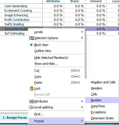
Right-click a measure. The right-click context menu appears.
Select Format and then select Number. The Format dialog box appears.
Select the measure and views for which you want to change the scaling.
Enter a value in the Scale option, as shown in Figure 4-4.
For example, if you enter 1000 as the scale factor, then all values in the view are displayed in thousands, meaning that a value of 35 actually represents 35,000.
When finished, click Apply and then Close.
You can use the scale factor for percentages as well. Enter a scale of 0.01 if you want to see values displayed as percentages, so that you see 19% rather than 0.19.
Your ability to edit multiple workbook cells and to easily move data in and out of the workbooks is essential to using RPAS to its fullest extent You can accomplish this by using the fill and clear functions. These are found in the Edit menu.
Use the clear feature to quickly clear the contents of cells in a view and set them to their NA value. With the clear function, you can clear one or more cells, a dimension level, or an entire slice.
Select the cells you want to clear. In Figure 4-7, the Wp Sales R cells for three months have been selected.
Select the Clear option in the Edit menu.
The selected cells are returned to their NA value, as shown in Figure 4-8.
The steps for clearing a dimension level vary depending upon which view you are in, outline or block. In block view, you can click Clear in the Edit menu just as you do when clearing cells. However, clearing a dimension level in outline view works differently if more than one level is in the selection.
To clear a dimension level in outline view, complete the following steps:
Select the cells you want to clear. In Figure 4-9, the entire Weekly Sales - Regular measure has been selected and two product dimension levels are selected, Fiscal Quarter and Fiscal Month.
Select Clear in the Edit menu or click Delete. The Clear dialog box appears.
Select the dimension level you want to clear and click OK. That dimension level clears in the background.
If you want to clear another dimension level, select it from the list and click OK. When you are finished clearing, close the Clear dialog box.
You can clear an entire slice, that is, all data shown in the view.
When you open the view, do not select any cell.
If cells are selected, you can deselect them by clicking a dimension tile, opening the Dimension dialog box, and then clicking OK to close it.
With no cells selected in the view, click Clear in the Edit menu.
A message appears, stating "Entire slice will be cleared because nothing is selected." Click OK.
The entire slice is cleared. If any read-only cells exist in the slice, you see a message informing you that the read-only cells have not been cleared.
If all selected cells are read-only, an error message appears, stating that none of the selected cells were editable and therefore the clear did not occur.
Use the fill feature to quickly populate many cells of a writable measure at a time. Depending on which view you are using, outline or block, one of the following dialog boxes appears.
|
Note: The fill feature cannot be used for hyper-dynamic pick lists because the list of available selections may vary from cell to cell. |
As shown in Figure 4-14, the outline view has additional dimension level fields. These are available whenever multiple dimensions are displayed in the outline view. You must choose which dimension level you want to fill with data.
To use the fill feature, complete the following steps.
Select what you want to fill. In Figure 4-15, the Wp Sales R measure for 100 Non-food Consumer Goods is selected. Its lower level has four positions within it.
With a cell selected, click Fill in the Edit menu.The Fill dialog box appears.
|
Note: If no cells were selected before the fill feature was invoked, all cells within the measure that is selected in the Fill dialog box are filled. The fill applies to the current slice only.If only a few cells were selected in the grid, only those selected cells are filled. |
Choose the measure you want to fill in the Measure field. If you select only one measure, as in the previous example, only one option appears.
Enter a value in the Fill Value field. The measure you select determines the type of data you can input as the fill value. For instance, if you choose a Boolean type measure, only true or false are available options for the fill value.
In the next field, select the level of the dimension that you want the fill to apply to. The name of this field varies according to the dimension you select.
Select the spread method to use to distribute that fill value among the lower levels that belong to the dimension level you select. For the spread method, choose among the following:
Replicate: Any value filled into an aggregate level cell is replicated exactly to every base level cell that comprises the aggregate total.
Even: Any value filled into an aggregate level cell is spread evenly among that cell's lower level constituents.
Proportional: Any value filled into an aggregate level cell is spread proportionally among all lower level constituent cells. This is based on the content of the cells before the fill.
Delta: The difference between the value pasted in the aggregated cell level and the original value of the aggregate cell level is spread evenly among all lower-level constituent cells.
|
Note: The Spread Method options are disabled when the base or lowest level of a dimension is selected. They are disabled because it is not possible to spread a fill value to lower levels if the lowest level is already selected. |
Decide whether you want the fill value to be spread to cells that currently have an NA value. If you select Do not spread to NA Value, the fill value data is not spread to lower level cells that contained an NA value before the fill. The NA values are left intact, and the aggregate data is spread to the remaining lower level cells.
|
Note: The Do not spread to NA value option is only enabled if the spread method option is enabled. |
Click OK when finished. The Fill dialog box disappears.
|
Note: If some of the selected cells are editable and some are read-only, a message appears stating that the read-only cells have been ignored. |
In the view, the new fill value appears in the cell. It is shown in italics because it has not been calculated or saved yet.
Click Calculate. The view refreshes and the fill value is now distributed throughout the lower levels. In Figure 4-17, the fill value is distributed evenly among the lower levels.
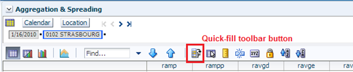
Use Quick Fill to replicate a value from one cell into other cells directly in the pivot table. To use Quick Fill, click the Quick Fill icon in the toolbar. The icon is shown in the following figure:
Quick Fill works in a similar way to copy and paste, except it copies the fill value from the top left cell of your selection and pastes it to the other selected cells. Your selection can include cells of the same measure or cells of different measures, as long as they are of a compatible type. Quick Fill is slightly different from Fill using the edit menu. Quick Fill can be used in outline or block mode.
|
Note: After using Quick Fill, you can do a calculation using the quick access toolbar or the calculate edit menu option. The updated cell value is sent to the server, and the associated cells are recalculated based on the calculation rules already configured. |
To use Quick Fill:
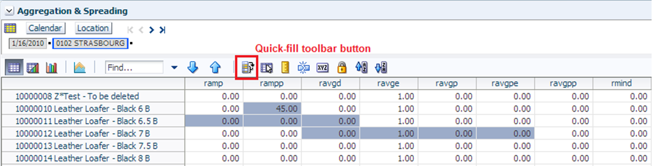
Make a selection in the pivot table where the upper left cell is the value you want to copy into the other selected cells. If you want to fill a different value to the selected cells, change the top left cell value.
In the example shown in the following figure, some of the cells are selected.
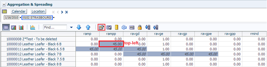
Click the Quick Fill icon, as shown in Figure 4-19.
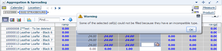
The system fills the data (top left cell's value) into the selected cells. If some of the selected cells do not match the data type of the fill value (data type of top left cell from the selections), or some of the selected cells are in read-only mode, the system ignores those cells and fills the rest of the cells.
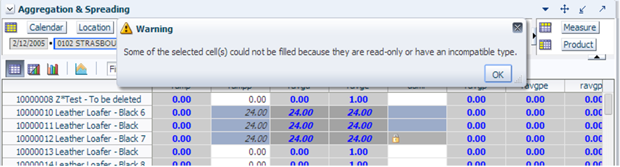
A warning message is displayed if some or all of the selected cells are ignored. Here are examples of a few of the warnings that may be displayed:
When the selection contains all editable cells, but some of them are a different data type.
When the selection contains editable, read-only, incompatible data type cells.
When the Quick Fill icon is clicked and one cell or no cell is selected in the view.
After you use Quick Fill, as with any other edit, values that have not been calculated or saved yet are shown in italics. If the top left cell has an undefined or ambiguous value, the fill operation is not completed and the following warning message is displayed: "Cannot Fill using a value that is ambiguous or undefined."
If you are in outline view with multiple levels selected, you can still use Quick Fill, but when a calculation is completed, the system may only honor the edit at one of the levels.
Quick Fill applies the fill value to the selected cells using the cells' default spread method, even when the value originally entered in the top left cell has a different spread method. For example, if you enter a value into the top left cell with a spread char, such as 10r, and quick fill that value to a selection, the filled cells do not use a spread method of r, unless that is their default spread method.
When you click the Quick Fill icon, the system fills the value to the selected cells that have same data type.
When you click Calculate, the view refreshes and the fill value is distributed throughout the lower levels. The spread method replicate (r) applies to the top left cell's measure only and values for rest of the edited measures use the measure's default spread method.
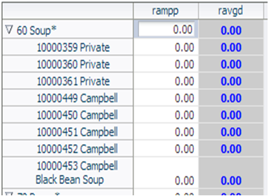
The following example illustrates how the spread method works. The example uses two measures, rampp and ravgd.
| Measure | Default Spread Method |
|---|---|
| rampp | RATIO |
| ravgd | delta (d) |
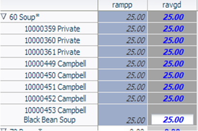
Figure 4-24 shows the initial cell values.
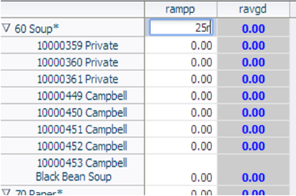
Figure 4-25 shows the 25r (replicate spread method) entered into the top left cell.
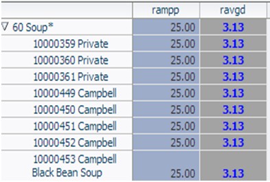
Figure 4-26 shows the results after you click the Quick Fill icon.
Figure 4-27 shows the cells after a calculate.
After you use Quick Fill, when the system fills the value to the selected cell and when you calculate, the replicate spread method is applied to the rampp measure and the measure's default spread method (ratio) is applied to the ravgd measure. The final results are shown in Figure 4-27.
In the view, you can make changes to the data cells. You can make the edits by directly typing or updating a value in the cell, copying and pasting, or by importing changes from a file. You can also lock a cell value by clicking the Lock icon on the View toolbar. This ensures that any calculation performed during the cell edits do not affect the locked cell values.
In the Fusion Client, you can modify workbook data in the following manner:
Click on the cell that you want to edit. Alternatively, navigate to the cell using the cursor keys and press F2.
After you enter or change the value in the cell, you can navigate to any other cell by double-clicking on that cell or using the following keyboard keys to navigate:
Enter to scroll down.
Shift + Enter to scroll up.
Tab to scroll right.
Shift + Tab to scroll left.
To learn how to modify data with math formulas, see Modify Data with Cell Formulas.
After you complete an edit action, you can revert the cell to the last calculated value using the Revert Cell option in the right-click context menu. The Revert Cell feature works on a cell-by-cell basis. When you click Revert Cell, the edited cell reverts to the last saved or calculated value. Changes up to the last saved or calculated value are available in the Undo list.
Protection processing is the process that makes some cells within a workbook read-only to ensure that during edits no conflicts occur within the RPAS engine in a Calculation Cycle. There are two types of protection processing:
Measure Protection Processing – Locks cells in all the displayed views based on the measures that have been edited.
Dimension Protection Processing – Locks cells based on the dimension intersections that have been edited.
Protection processing runs each time when a workbook with any locked cell or measure is opened, a cell is edited, a cell or measure is locked, and after each cell revert action. It runs only once when a group of cells is updated in one action. Protected cells or measures appear highlighted in a different color in the view. This is a configurable feature.
In measure protection processing, cells become read-only when you make changes to enough measures. This ensures that there are no more possible changes that may cause conflicts.
For example, consider six measures (A, B, C, D, and E) set up with the following two rules:
Rule 1 - A = B + C
Rule 2 - B = D + E
In this scenario, both A and B are read-only before any edits are applied. Although B appears to be editable, since there are no reciprocal expressions for B's relation to D and E, it is not editable. Measures C, D, and E, however, are editable.
Typically, rule definitions are set up to include all equivalent derivations of any expression. This ensures that you can edit all of the measures contained in any expression in the rule.
Considering the previous example, Rules 1 and 2 will be configured as:
Rule 1 A=B+C, B=A-C, C=A-B
Rule 2 B=D+E, D=B-E, E=B-D
In this case, all measures are editable before you make any changes and the measures remain editable based on the edits you make.
Measure protection processing locks all instances of a measure when any position of the other measures in the rule are edited.
For example, consider the Rule 1 in a typical Product, Location, Calendar dimension.
When you edit the measure B for product 1, location 1, and week 1 and measure C for product 1, location 1, and week 2, the measure A becomes read-only for all products at all locations in every week.
Changes to cells at the aggregated levels occur during a spread action that changes values down to the base intersection of a measure. Dimension protection processing protects the intersections (combination of levels) to ensure that all changes made during the spread do not affect such a spreading path.
Considering the typical retail dimensions, the process applies at product:color-location:store-calendar:week and product:style-location:region-calendar:month. These two intersections are on the same path from the root to leaf. If the location dimension has roots for both region/state and Store Volume, any edit to a cell in the Volume Group dimension causes all cells included in an intersection with a company/region/state/city to become read-only.
Dimension protection processing changes to the intersection of dimension and level are processed, and edits are allowed to cells as long as the edits are on one path from the root to the leaf level.
If a measure has been set up to have dimension values as inputs, the measure cell displays a drop-down list of positions, as shown in Figure 4-29.
For example, a Week Mapping measure can be configured to have the week position of the Calendar dimension as an input. The selection of the dimension is configured in the domain configuration for a measure.You can either select a value from the list or click Search at the bottom of the panel, as shown in Figure 4-30.
The Search link launches the Search dialog box, where you can search for specific values. The search dialog box automatically opens on the Advanced search option (Figure 4-31).
To use the basic search, click Basic. The Search dialog box refreshes with the basic search tools (Figure 4-32).
The cut, copy, and paste features provide flexibility to edit the workbook according to the business needs and transfer data from external applications (such as Microsoft Excel) to the system as well as from RPAS to those external applications.
To apply the operation, select data from the view. After selecting the appropriate cells, you can cut, copy, and paste. For more information, see the Cut, Copy, and Paste sections or Cut, Copy, and Paste Special and Copy to External and Paste from External.
|
Note: The maximum number of cells that can be copied, cut, or pasted is limited by memory. These operations should not be used to export entire workbooks. For more information, see Export.You cannot cut or copy multiple cells when an edit is in progress. While an edit is in progress, only the current edited text is copied. To copy multiple selected cells, click Escape to exit and then select the multiple cells again. |
Date and Time Data Handling in Cut/Copy/Paste Operations
Since date and time measures can be formatted to display no time, 12-hour formatted time, or 24-hour formatted time, date and time data is handled differently when it is cut, copied, or pasted.
When date and time data is cut, copied, or pasted internally, the full date and time data is captured, regardless of whether the measure is formatted to display the full date and time. If the measure is formatted to display no time and no time is entered in the cell, RPAS stores the time as 00:00:00 and is displayed as 12:00:00AM in 12 hour format and 00:00:00 in 24-hour format.
When date and time data is cut, copied, or pasted externally, you have two options:
The As displayed option copies the data with its formatting
The Raw value option copies the data without its formatting
If time data is stored in a cell but is not displayed due to the measure's formatting, when that data is pasted to a 12-hour or 24-hour formatted cell, the time data is reformatted to match the destination cell's formatting. Similarly, when time data is copied from a 12- or 24-hour formatted cell to a cell with no time formatting, the data is pasted but the time is not displayed. If a time is copied from a 12-hour formatted cell and pasted to a 24-hour one (or 24-hour to a 12-hour), the data is converted automatically during the copy/paste operation.
For more information about time formatting, see Modifying Date/Time.
Use this procedure to copy and remove data from the cells of a view in order to move the data to another view or other applications. Note that data created from deferred calculations can be cut.
|
Notes: You cannot cut data from non-editable or read-only measures. |
To cut data, complete the following steps:
Select all data cells in the pivot table that you want to cut.
To cut the data and copy it to the clipboard, use one of these three methods:
From the Edit menu, click Cut.
Right-click and select Cut from the right-click menu.
Use the shortcut command Ctrl + X.
Data from the selected cells is copied to the clipboard. The selected cells now contain NA values.
To paste the data to other cells or to another application, see the Paste section.
|
Note: To remove the last deferred entries after using the cut option, right-click and select Revert Cell from the right-click menu. Or, use the shortcut option Ctrl + Z. You can also select the Undo option. |
Use this procedure to copy selected data to the application clipboard. Unlike the cut function, the copy function does not clear the data from the view cells. It keeps data in a clipboard that you can use to transfer data within RPAS as well as to an external application such as Excel. It also helps you to transfer large amount of data easily. When cells are copied, only the unformatted textual content is transferred.
When data is copied from a cell to the clipboard, the string representation of the cells is copied to the clipboard so that it can be pasted into either other cells in the pivot table or to external applications. Data containing deferred calculations can also be copied. There is no need to invoke Calculate before copying.
Table 4-2 shows what is actually copied to the clipboard, based on cell (measure) type.
Table 4-2 Copied Data
| Cell (Measure) Type | Behavior |
|---|---|
|
Boolean |
True, or checked, values are copied as 1. False, or unchecked, values are copied as 0. |
|
Date/Time |
The formatted date is copied and visible in the cell. If the measure is configured to contain the time, the time is copied as well. |
|
Integer |
The formatted number as displayed in the cell is copied. Prefixes and suffixes, such as $ or %, are copied as well separators. |
|
Picklist |
The value displayed in the cell is copied. |
|
Real |
The number as displayed in the cell is copied. The format, such as $ and %, is copied as well. |
|
Single dimension |
The value as displayed in the cell is copied. |
|
String |
The value as displayed in the cell is copied. |
To copy data, complete the following steps:
Select all data cells in the pivot table that you want to copy.
To copy the data to the clipboard, use one of these three methods:
From the Edit menu, click Copy.
Right-click and select Copy from the right-click menu.
Use the shortcut command Ctrl + C.
|
Note: If no cells are selected, the Edit menu and right-click options are grayed out. If no cells are selected when the Ctrl +C method is used, a warning message appears that states, ”No positions have been selected for this operation.” |
The selected cells are copied to the clipboard.
After you have copied or cut data from a view, you can paste the data to other cells within the RPAS Fusion Client or you can paste it to an application such as Excel. The Paste option pastes the data that was last placed on the clipboard into the selected cells.
|
Note: Although non-contiguous data cells can be copied, they cannot be pasted as non-contiguous cells. Data copied from non-contiguous cells does not maintain the pattern in which it was copied. For information about selecting non-contiguous cells, see Select a Group of Non-Contiguous Cells. |
To paste data, complete the following steps after you have copied or cut data from another location:
Select the cells into which you want to paste the data.
To paste the data into the cells, use one of these three methods:
From the Edit menu, click Paste.
Right-click and select Paste from the right-click menu.
Use the shortcut command Ctrl + V.
|
Note: If protection processing does not allow data to be pasted into the selected cell, the paste operation is aborted. |
The following sections describe the cut, copy, and paste special features.
You can also cut data at the base level or higher level intersection across page slices. If multiple levels (such as product group or style) are represented in the pivot table selections, the cut option is performed at the lowest level actually selected. After data is cut from the selected cells, it can be pasted into other selected cells in the pivot table. To cut data, complete the following steps:
Select all data cells in the pivot table that you want to cut.
From the Edit menu, click Cut Special.
The Cut Special menu appears.
Select from the following options:
Cut all slices: This option is enabled only if the current workbook view contains more than one page slice. Otherwise, this option is disabled. When this option is selected, the cut operation behaves as if all positions in the slice dimension's levels were selected prior to the cut. If the box is left unchecked, only the data from the current slice position is cleared and copied.
Cut selected level: This option cuts only the selected level of data.
Cut at base level: This option allows you to cut the data at the measure's lowest intersection.Although the cut function is performed at the base level, it seems that the aggregated level data has been cut since the data is rolled up.
You can also copy data at the base level or higher level intersection across page slices. After data is copied from the selected cells, you can paste data to other selected cells in the pivot table. This feature allows you to view data at an aggregate level while copying data at a dimensional level not currently displayed or while selecting data from the current slice while copying data from all slices. You can copy data at the base level only or copy from all slices without selecting the base level data or without selecting data from entire slices.
|
Note: Data copied using the Copy Special option is not copied to the clipboard. It is copied to the RPAS server. |
To copy data, complete the following steps:
Select all data cells in the pivot table that you want to copy.
From the Edit menu, click Copy Special.
The Copy Special menu appears.
Select from the following options:
Copy all slices: This option is enabled only if the current workbook view contains more than one page slice. Otherwise, this options is disabled. When this option is selected, the copy operation behaves as if all positions in the slice dimension's levels were selected prior to the copy. If the box is left unchecked, only the data from the current slice position is copied.
Copy selected level: This option allows you to copy the level of data shown in the pivot table. The base level data from which the displayed data is created is not copied.
Copy at base level: This option allows you to copy the base level data (the measure's lowest intersection), which may not be displayed in the pivot table. If this option is not selected, the data is copied for the selected dimension level only.
The selected data is copied to the RPAS server. It is not copied to the clipboard. You can paste the copied data to other selected cells in the workbook multiple times. The copied data is available to the RPAS server until the workbook is closed.
Use Paste Special to view data at an aggregate level while pasting it at the base level, which is not displayed in the current slices. It provides a dialog in which you can specify options for specialized paste functions.
If the levels of multiple dimensions are represented in the pivot table selections, the default paste option is performed at the lowest level.
To use special paste, complete the following steps:
Before using paste, you have placed data in clipboard using Cut Special or Copy Special from the Edit menu.
Select Paste Special from the Edit menu.
The Paste Special menu appears.
Select from the following options:
Paste all slices: This option pastes data to all slices. If this option is not selected, data is only pasted to the currently displayed slice position.
Do not paste NA values: If this option is selected, NA data that has been cut or copied is not pasted into the current selection. Whenever the system encounters an NA value in the copied data, that value is ignored and the data cell being pasted keeps its original value. In other words, when this option is selected, the current pivot table data is not overwritten by NA values.
Paste selected level: This option only pastes data at the level of data shown in the pivot table.
Paste at base level: This option is enabled only if none of the base level measures are selected before the paste. Use this option to paste data at the base level, which may not be currently displayed in the workbook. You can view data at an aggregate level while pasting it at the base level.
Click OK. The selected data is pasted.
Use the Copy to External and Paste from External options to copy and paste data from the system clipboard when the browser's security restriction prevents the Fusion Client from copying to and pasting from the clipboard. These options are necessary for Mozilla Firefox and Google Chrome.
Use the Copy to External feature when data from the pivot table must be copied to an application other than RPAS Fusion Client, such as Microsoft Excel or Notepad. To use the Copy to External feature, complete the following steps:
Select the cells to be copied in the pivot table.
Click the Copy to External option in the Edit menu.
A dialog box appears, containing the copied data from the pivot table. The data is formatted correctly and is selected in a text field.
To execute the browser's copy command, select the copy option from the browser menu or click CTRL+C. This copies the selected text from the text field to the system clipboard. Click Close.
The data can then be pasted into another application. It can also be pasted into the Fusion Client using the Paste from External option.
Use the Paste from External feature when you need to paste data into the Fusion Client from the system clipboard.
To use the Paste from External feature, complete the following steps:
Copy the data in the correct format from another application.
Select the area to paste in the pivot table by selecting the upper left hand corner of the paste area or the exact cells to be pasted into.
Click the Paste from External option in the Edit menu.
A dialog box appears, containing an empty text field.
To paste the clipboard data into the text field, use the browser's paste command from the browser menu or click CTRL+V.
Click Paste in the dialog box to paste the data in the selected pivot table.
Read-only measures are defined during the domain configuration process. The read-only status can be set at both the base intersection and aggregate levels. Read-only measures are indicated as non-editable cells based on measure information retrieved when the workbook is opened.
Read-only cells by default have a gray cell background color. This same default color is used to indicate protection processing protected cells and elapsed cells. If the visual indicator for read only is changed to be different than the visual indicator for protected cells and the cell is both read-only and protected, then the cell will display the visual indicator for protected cells. These cells are not editable from the RPAS Fusion Client.
In addition to read-only workbooks and measures, the RPAS Fusion Client also provides a locking function in order to protect information. The locking function can be used on cells, measures, and positions.
Cell locking is available for any editable cell and invokes protection processing.
Measure locking is available for any measure and invokes protection processing.
Position locking is available for non-calendar dimensions and does not invoke protection processing.
|
Note: Locks are not recognized by operations such as custom menus and refresh. Locks are only recognized when a workbook calculation. is done. |
Use the cell locking feature to lock one or more editable cells in the pivot table. When a table cell is locked, calculations performed as a result of data manipulations do not affect the locked data values. This functionality allows you examine various what-if scenarios to determine the best course of action for planning or forecasting.
The RPAS Fusion Client iterates through the selected cells by measure, then by column, then by row. Locked cell information is immediately transferred to the RPAS server. The locked cell information is saved with the workbook and locked cells continue to be locked when the workbook is reopened.The locked status of a cell is indicated by the presence of a picture of a lock on the left side of the cell. After an eligible cell is locked, the system determines whether the remaining table cells are eligible or ineligible for locking. For instance, if all the child cells of any parent cell are locked, the parent cell cannot be locked. Instead, any edits to the parent cell are spread to the child cells based on the ratio of the values locked into the cells. If a cell becomes ineligible for locking, the right-click menu associated with that cell does not contain the Lock option. Furthermore, any read/write cells that become ineligible for locking are made read-only.You may choose to lock a data cell at any time to protect that cell from forced recalculations as a result of data manipulation elsewhere in the workbook. For example, you may want to see the effect of a change to sales value on inventory levels without forcing a change to receipts. Or, you may want to change sales value at an aggregate level (such as month) and spread the result to only three of the four weeks that comprise that month. In this case, you can effectively hold the second week's sales value constant while spreading the aggregate-level increase among the remaining three weeks.
Protection processing executes against locked cells as if they were edited to their current value. Cell locks do not appear in the Undo list, which appears next to the Undo icon in the toolbar when more than one edit has been made. In addition, cell locks are not affected by the Undo option from the menus. Only cell value edit changes appear in the Undo list. Cell lock or unlock actions do not force a calculation cycle to execute.
Use the measure locking feature to simultaneously lock all of the cells that are associated with a given measure in a view. A measure can be locked or unlocked when the header cell of the measure dimension is selected. As with individual cell locking, the locked status of each cell in the measure is indicated by the lock picture on the left side of each cell.
Locked measure information is immediately transferred to the RPAS server. The locked measure information is saved with the workbook, so locking measures enables the save features of the workbook. The locked measure information is saved with the workbook and locked measures continue to be locked when the workbook is reopened.
Protection processing executes against a locked measure as if the measure has been edited to the same value.
If multiple measures are selected, they are locked or unlocked in row or column order. A measure may be locked even if it is already protected by protection processing.
|
Note: You can only make a selection at one level in the headers of a multidimensional header. Lock and unlock apply to the selected measure only. Locked measures are designated by a lock icon in the header text of the measure and in its cells. |
Use position locking to lock all measures in all displayed views along one or more positions of non-calendar dimensions. Cells along unlocked positions are still editable and can also change as a result of calculations. Locked positions are designated by a lock icon in front of the position name. The cells of the locked position are shaded as read-only.
Protection processing does not run against cells locked by a position lock. Unlike cell locks, a parent position becomes locked if all its children are locked. A parent position becomes unlocked if any of its children are unlocked. Hidden children are considered when deciding if a parent position becomes locked. Unlocking or locking the parent unlocks or locks all the children. Hidden child positions are treated in the same way as visible children. Unlike a measure lock, the lock indicators do not show up in each of the cells, only in the header cells, even though the cells are displayed as read-only.Locked position information is immediately transferred to the RPAS server. The locked position information is saved with the workbook, so locking positions enable the save features of the workbook. The locked position information is saved with the workbook and locked positions continue to be locked when the workbook is reopened.A position cannot be locked when locking it affects an edited or locked cell. A warning modal dialog is displayed and asks you to revert the affected edits and calculate the workbook or cancel the position locks. You are warned if a cell lock is affected and given the choice of canceling the position lock or unlocking the affected cell locks and continuing. If both edits and cell locks are affected, then you see both dialogs, with the edit dialog appearing first. If you cancel the position lock from either dialog, then no action is taken against either locked or edited cells.
You can initiate locks by selecting a cell, measure, or position within the pivot table and then selecting one of three options to initiate a lock or unlock action. Locking and unlocking can be done through the following:
One way that you can lock or unlock a cell, measure, or position is by using the right-click context menu. Depending upon what is selected, the context menu determines whether the Lock or Unlock option is shown.
To lock using the context menu, complete the following:
Select a cell, measure, or position. After it is selected, it is shaded.
Right-click the mouse. The context menu appears. If the cell, measure, or position is not already locked, the Lock option appears in the menu.
Select the Lock option.
The selected item or items show a lock symbol.
You can lock a cell, measure, or position by using the Edit menu. The Edit menu contains several locking options:
Lock
Unlock
Unlock All Cells
Unlock All Measures
Unlock All Positions
To lock using the Edit menu method, complete the following:
Select a cell, measure, or position. After it is selected, it is shaded.
From the Edit menu, click the Lock option.
The selected item or items show a lock symbol.
To unlock using the Edit menu method, complete the following:
Select the cell, measure, or position that is locked.
From the Edit menu, click Unlock.
Or, if you want to unlock all cells, measures, or positions, select Unlock All and choose the type you want to unlock.
You can lock a cell, measure, or position using the Lock icon in the toolbar. If some selected cells are already locked, they are ignored. If all selected cells are already locked, then the selected cells are unlocked instead of locked. If an error occurs when any of the selected cells measures or positions are locked, then an error message will be displayed and all of the applied locks will be reset. Cells that were already locked when the lock action started will remain locked.
To lock using this method, complete the following:
Select a cell, measure, or position. After it is selected, it is shaded.
Click the Lock icon in the toolbar.
The selected item or items show a lock symbol.