| Oracle® Retail Predictive Application Server User Guide for the Fusion Client Release 16.0 E81120-03 |
|


 Previous |
 Next |
| Oracle® Retail Predictive Application Server User Guide for the Fusion Client Release 16.0 E81120-03 |
|
Previous |
Next |
Easily sorting and finding data is essential when working with workbooks that contain thousands of items, hundreds of locations, and an endless number of dates. Being able to put this data in a logical order or find a specific piece of information is what makes planning possible.
This chapter describes the ways you can sort, find, and query data:
There are two kinds of sort: simple sort and attribute sort. Both can be used to put the data in a meaningful order.
You can sort positions in a level by using the sort icons on the toolbar or the arrows that appear on column headers. The positions are sorted based on the values of a measure's slice for that level. This sorting can be done without defining additional attributes.
The sort occurs along a single measure, using only a single level in the sort. The sorting is limited to the current view, providing the user an ability to see the same data sorted differently in different views. Sorting is only available in the pivot table or split view. It is not available in the graph view.
|
Note: A slice is valid if it involves only one measure and if it has a unique value for each position along the level being sorted (meaning that one position along all other dimensions in the measure's intersection has been selected).A simple sort cannot be applied to positions in a dimension along the page axis. However, you can pivot the desired dimension to either row or column axes, execute the sort along the desired slice, and then pivot the sorted dimension back to the page axis. |
After you have selected the desired valid slice of measure data that you want to sort, the sorting arrows are enabled on the toolbar and in the columns, as shown in Figure 11-1.
After you click one of the sort arrows, the selected positions are sorted according to the measure's values in the selected slice.
The Sort Ascending icons in the toolbar and columns order the data so that the lowest number appears at the top of the list and the highest at the bottom. After the data is sorted, the column header is shaded gray and the Sort Ascending arrow is shaded dark gray, as shown in Figure 11-2.
The Sort Descending arrows order the data so that the largest number is at the top. Again, after the data is sorted, the column header is shaded gray and the Sort Descending arrow is shaded dark gray (Figure 11-3).
Sorting should be reapplied after operations that do not change the data. If you show or hide positions, change the rollup, or switch the mode from outline to block view or vice-versa, you should reapply the sort. Since a pivot operation resets the selected sort slice, you must reselect a valid slice and sort again. If you use the View Attributes and Sort tab to perform a attribute sort, the simple sort is overridden. Previous sorts (either attribute-based or simple sort-based) are not maintained after a new simple sort. Data editing operations like calculate, update, or refresh do not reapply the sort, and the positions remain in the last sorted order.
If you edit a cell and attempt to sort using the toolbar icon, a message appears that states that the edited cells need to be calculated before the sort operation can take place.
You can choose to calculate, revert, or cancel:
Calculate: The positions are sorted after the calculate operation is performed.
Revert: The edits are reverted and the sort is performed.
Cancel: The sort operation is canceled.
If you have edited the cells and attempt to sort using the column header icon, the page refreshes without applying the sort and the header no longer displays the icon to sort. If you perform other operations such as show and hide after the edits that have caused the page to refresh, the sort icon does not appear in the column header until the edited cells are calculated.
You can sort data by mousing over the pivot table column headers to make the ascending and descending sort icon appear.
Click the icons to sort the positions along the row-edge based on the vales of a measure's slice for that dimension. The column is highlighted and the column header displays a selected sort icon (ascending or descending) based on the sort direction.
The sort icons do not appear on the column headers if the slice (with the selected column) is invalid. For example, when the measures are on the row edge, the sort icons do not appear on the column headers. Also, when there is more than one dimension on the column axis, the sort icons appear only on the inner layer.
The sort icons in the toolbar are enabled if there is a valid slice involving a single measure being selected. Select either a column or row and click the one of the sort icons. The toolbar icons are more useful for sorting the rows.
The selected position is sorted according to the measure's values in the selected slice. If the rows were sorted, only the row appears selected. If a column was selected, a sort icon appears in the column header. If you select an invalid slice, for instance, multiple rows or columns, the sort icons are enabled but clicking them results in an error message that states the selected slice is not a valid slice for sorting.
You can sort in either the outline or block mode. Sorting in the outline mode sorts all the positions as well as the positions within those positions. Sorting in block mode, however, only sorts the highest aggregate position.
If the pivot table is in outline mode, that is, it displays aggregate levels of the dimension in separate rows or columns in the same grid, the aggregate positions as well as the positions within the aggregate positions are sorted.
In Figure 11-8, note how the 5 Pocket Capri position is listed first because it is larger than both the 5 Pocket Frayed Jeans and Bohemian 5 Pocket Jeans groups. Then, within the 5 Pocket Capri group, the style/sizes are listed in order of greatest to least, the "Antique 10 An" being the largest of all the departments.
If the pivot table is in block mode, that is, it displays the dimension levels in separate rows or columns but not the aggregate levels, the simple sort still orders the aggregrate levels as well as the dimension levels within them.
In Figure 11-9, note how the 5 Pocket Capri, 5 Pocket Frayed Jeans, and Bohemian 5 Pocket Jeans groups do not have an aggregated number in the column. Nevertheless, the groups are still ordered greatest to least, as are the style/sizes within those groups.
When the positions are sorted on a specific slice, by default the positions stay in the previously sorted order as you page through the positions along the page-axis. In other words, the positions are not resorted based on the new selections in the page-axis. If you want to reapply the sort when paging through positions along the page-axis, you must enable the Resort Positions on Pagination option in the View menu.
For example, there are two slices that display the sales of five stores: one slice displays data for the denim 5 pocket capri, the other displays data for the antique capri. Before sorting, the five stores are listed in alphabetical order, as shown in Figure 11-10. When the user scrolls from one slice to the other, the stores stay in alphabetical order.
When a user sorts the denim slice by descending order, the stores are reordered so that the store with the highest sales, Berlin, is at the top. If the user scrolls to the antique slice, Berlin is still at the top even though the Chicago store has the highest sales. This is because the positions stay in the same order by default. They are not resorted according to the data. This is shown in Figure 11-11.
On the other hand, if the Resort Positions on Pagination feature is turned on, the positions are resorted according to the data. The Resort Positions on Pagination option is located in the View menu.
When the Resort Positions on Pagination feature is turned on and the first slice is sorted by descending order, when the user scrolls to the next slice, it too is sorted, as shown in Figure 11-12.
|
Note: Simple sort cannot be applied to positions in a dimension along the page axis. However, you can pivot the desired dimension to either row or column axes, execute the sort along the desired slice, and then pivot the sorted dimension back to the page axis.The Resort Positions on Pagination option is saved with the workbook formatting. For more information about formatting and how formatting is saved, see Saving Formats. |
If you want to undo a sort, right-click and select Undo Sort from the right-click context menu.
You do not need to select the exact slice; any slice on the sorted dimension renders the Undo Sort option. After you select the Undo Sort option, the simple sort is no longer applied and the positions appear in the original sort order that was shown when the view was first opened.
An attribute is a piece of information that further describes a position at a given level. For example, the SKU level of the product dimension could have three attributes associated with it: label, color, and price. This means, any SKU in this product dimension could have attribute values of:
LABEL:SKU00012 - Cashmere Sweater
COLOR: Pale Blue
PRICE: $62
Label is the only attribute that is required, but positions in a level can be described with any number of attributes. After they are established, attributes can be displayed in the view if desired. The dimension's attributes can also be used to decide display sort order for positions within that level.
But before you can sort by attributes, you need to select the desired attributes to appear in the view.
To see the available attributes that you can sort by, complete the following steps:
|
Note: You use the Show Attributes and Sort tab to determine which image attributes are visible in the UI. For more information about images, see Chapter 2, Chapter 13, and Chapter 14. |
In an open view, click the dimension tile of the dimension that you want to sort by an attribute. In Figure 11-15, the Location dimension has been selected.
The Dimension window appears. Click the Show Attributes and Sort tab.
In the Show Attributes and Sort tab, the available attributes for the dimension are listed in both the Available Attributes and Sort Attributes sections on the left. The attributes currently shown in the view are listed on the right. These attributes have a check mark beside them.
Select the attributes that you want to appear in the view from the Available Attributes section at the top.
Either click the right arrow to move the attribute to the Visible Attributes box on the right side or drag the attribute to the right side.
Repeat the same process for the attributes you want to sort by moving them to the Sort Attributes section at the bottom.
When you are finished, click OK. This saves your changes and closes the window.
If you want to make additional changes on other tabs in the Dimension window, click Apply instead. This saves your changes but leaves the Dimension window open so you can go to other tabs.
The attributes now appear in the workbook as shown in Figure 11-17.
If you have selected image attributes to appear, they will be displayed as well. You can hover over the image in order to see the position and image label.
In the Fusion Client, you can display attributes in both the outline and block views.
In the outline view, you can view the attributes in either the row edge or the column edge. In outline view, for each dimension, the first layer displays attributes with display order 1 merged across levels. This layer also features the expand and collapse icons. By default, after the first layer, each displayed attribute is rendered as a separate layer.
You can view attributes in two places in the outline view: the row edge and the column edge.
In the outline view, the default ordering of displayed attributes across levels is from higher to lower levels. For example, the attribute from the higher district level is displayed, first followed by the lower store level.For each dimension, the first layer always features the expand/collapse icons. In addition, the label itself is an attribute, and you can choose to display it in any order or hide it altogether (as long as there is at least one attribute displayed for each level). For example, you can choose the label attribute for both the store and district levels as second in display order, with SKU Label reordered before District Label.
Attribute labels can be combined with levels and shown as Level Label (Attribute Label) format. For example, the Store (Fmt) shown in Figure 11-19. The attribute label hovers above the layer. However, hovering over the first layer just displays the dimension label.
You can choose to display multiple attributes as a single layer by using the merge option in the right-click context menu. After you have merged two attributes together, you can split them using the split option in the context menu option.
|
Note: The Merge and Split feature is only available in the outline view, not the block view. |
To merge two attributes, complete the following:
Right-click one of the attributes you want to merge.
In the context menu that appears, select Merge and then select the other attribute from within the Merge menu. See Figure 11-20 for an example.
The attributes are merged together and appear in the same row or column. Note how the Store Count and Store Format attributes are now in the same column in Figure 11-21.
Only attributes belonging to different levels can be merged. You cannot perform Merge and Split actions on the first layer in the outline view because this layer displays the first attribute across the merged levels.
To split two attributes that have been merged, complete the following:
Right-click a merged row or column.
In the context menu, select Split and then select one of the merged attributes from within the Split menu.
In the outline view, you can merge or split attributes across levels using the right-click context menu. However, the first layer would always display attributes with display order one merged across levels. In addition, you cannot merge attributes that belong to the same level.
|
Note: The merge and split feature is session-only and is lost after you close the session. |
In the block view, each layer renders one attribute and all the displayed attributes for a level are shown consecutively in the user-selected display order, as shown in Figure 11-23. The first layer in each dimension features the expand and collapse icons.
In the block view, the attribute ordering always follows the display order you select. You can reorder using drag-drop, but that is the same as using the View Attributes and Sort tab to change the attribute display order.
You can also right-click an attribute and hide the block view. This completely removes the associated layer from view.
As in outline view, the expand and collapse icons are on first layer for each dimension. You can display the label attribute in any order or even hide it altogether (as long as there is at least one attribute displayed for each level).
You can also see the attributes of a dimension that is in the page edge. The attributes are displayed on the page edge and are separated by a bar separator. The attribute labels are added to the level display when you mouse over.
In both the outline and block views, you can reorder attributes across levels by dragging an attribute row or column to a different location.
|
Note: The reordering feature is persisted in the session only. After you close the session, the new order is lost. |
To change the order of attributes, complete the following:
Mouse over the area above the row until the attribute label appears.
Click and drag the attribute label. As you move the attribute row or column, the available locations where you can drop the attribute are shaded gray.
When the location where you want to move the attribute is shaded gray, drop the attribute.
You can sort positions in a level using any of the level's attributes. Use the View Attributes and Sort tab to choose the attributes used for sorting. You can also define sort direction (ascending or descending) and the order that the attributes you select are to be applied during the sorting process. For example, the SKUs in the product dimension can be sorted primarily by price, and then within those prices by label.The sort is applied dimensionally across multiple levels. For example, if the product dimension contains the levels company, division, class, style-color, and SKU, the positions within the company level are sorted first by the selected sort attributes for company, and then positions within each division, applying the division's selected sort attributes, and so on.As with display, if an attribute is the default sort attribute for a level, the default sort is always applied if you have no other selection. The attribute-based sort order does not override any current simple sort selection, unless you:
navigate to the View Attributes and Sort tab and click OK or Apply. This reapplies the attribute-based sort even if you do not make any changes on this tab.
select Undo Sort in the right-click context menu.
For measure dimensions, the sort order you define is applied by default. You can choose the Disable User defined Sort Order option on the Show/Hide tab to disable the default behavior.
|
Note: The RPAS Fusion Client displays a warning that when all sort attributes are removed from the Show Attributes and Sort table of the dimension pop-up, the values are displayed in default sort order. For the RPAS Fusion Client, the default sort order is Label. It is not the order returned from the RPAS Server. To get a guaranteed sort order, create a sorting attribute and populate it with values. |
Use the find feature to search for words, partial words, or phrases within the rows, column, and page axis of an active view. The search does not include the data within the view.
The find feature locates the phrase you looking for and shades it gray. If the matched position is not visible because it is hidden under a scroll bar, the view is automatically scrolled to reveal it. The search is performed through collapsed or hidden positions. When a matched position is found, the parent is expanded and the matched position is shaded gray.
The find feature can be accessible four ways:
The Find option in the right-click context menu
The Find option in the Edit menu
The shortcut Ctrl + F
The Find field in the view toolbar
To use the find feature from the right-click context menu, complete the following:
Right-click a measure, position, or attribute label to see the right-click context menu. Note that right-clicking on a data cell does not activate the find feature in the right-click context menu.
Click Find.
The Find window appears.
Enter the following:
Search For: Enter the text you want to find.
Match Case: Select this option if you want the search to locate text that use the same case as the text you entered. Leave it unchecked if you want the search to find all text that match yours, regardless of case.
Whole word Only: Select this option if you want the search to find the text in a whole word rather than a partial one.
For example, if you are searching for the letter U and you select the Whole word Only option, then the search will find the Wp BOS U measure, but it will not find the letter U within the Wp BOS AUR measure.
Only within...: Select this option to search in a variety of ways:
Search for the text only within one or more measures, positions, or attributes that you right-clicked in Step 1. When this option is selected, the search ignores all matches outside of those measures, positions, or attributes.
Search within multiple positions by selecting more than one member to search through.
Find the text within a specific member and within its own dimension.
Find the text within a specific member and within another dimension.
In outline mode, use this option to find positions within different levels (style, SKU).
In block mode, use this option to find positions within the same level (either style or SKU).
Dimension: Specify what dimension you want to search within. This is a required step.
Levels: Specify which level of the dimension you want to search within. You can choose a specific level or you can choose All to search all levels. The search is performed level by level, not through parent and child. For example, when there are two levels, style and SKU, the search is performed in the style level first and then the SKU.
When finished, click Find Next. The view refreshes. If a match is found, it is shaded gray.
Click Find Next to see the next match. You can click Find Previous at any time to see matches you have already seen.
If a match is not found, the following message appears:
|
Note: A similar message appears when you reach the end of the search and asks if you would like to start the search again. |
Using the Find feature from the Edit menu or Ctrl + F works in the same way as the right-click context menu.
After you have opened a workbook, click Find in the Edit menu or enter Ctrl + F. It is not necessary to select anything in the view.
The Find window appears. Enter the information as described in Step 2 of the Find Using the Right-Click Context Menu section.
|
Note: If no position was selected in the workbook, the Dimension field will not have a dimension automatically selected. You must select a dimension from the list to perform the search. |
When finished, click Find Next. The view refreshes behind the Find window.
The Find field within the View toolbar is a quick alternative to using the Edit or Context menus.
To use the find option in the workbook toolbar, complete the following:
Enter a phrase in the Find field.
Click the Find Options arrow to manage the search parameters. This is an optional step. If you skip this step, the search is performed on all dimensions.
Dimension: Select the dimension you want to search in or select All to search all dimensions.
Match Case: Check this option if you want the matches to have the same case that you entered.
Whole word Only: Check this option if you want to find the text in a whole word rather than a partial one.
Click either the Previous or Next arrows to begin your search.
Position queries are preconfigured rules that filter data so that only positions that fulfill the requirements of the query are shown in the view. Position queries are configured in RPAS Configuration Tools by an administrator. For instance, if an administrator has configured a position query to filter for the stores with sales greater than $3500, you can turn on that position query to display only those stores.
The dimension that the query is based on must be in the page edge (Z axis). This is known as the driving dimension. The dimensions in the X and Y axes are known as the query dimensions. The data in the query dimensions is based on the current position of the driving dimension.
When a position query is applied to a view, the positions in the query dimensions
(X and Y axes) that fulfill the requirements of the query for the particular position of the driving dimension (Z axis) are the only ones shown in the view. All other positions are automatically hidden.
When more than one driving dimension is present, all of the driving dimensions have to be in the Z-axis for the position query to execute. If one or more driving dimensions are taken out of the Z-axis and placed in the X or Y axes, associated position queries are not executed. A given view can have more than one position query, driven by one or more dimensions in the Z-axis and driving different dimensions in the X and Y axes.
You can configure a worksheet with the Lock PQD dimensions. With these worksheets, you cannot move a driving dimension off the Z-axis. If the PQD's driving dimension is not on the page edge, or the driving level is not visible on the page edge, the PQD will not be visible until that is true, at which point the Lock will take effect.
When the position query filter is turned off, the icon appears flat. When you mouse over the icon, the roll-over text says ”Filter [Rule].”
When a position query filter is turned on, the position query icon is depressed. When you mouse over the icon, the roll-over text says ”Remove filter for [Rule].”
If you have a workbook that is configured to have a position query, you can filter to view only the positions that fulfill the requirements of that query.
For this example, a Sales Total workbook has been configured to include a position query to filter locations with the Store measure selected. As shown Figure 11-36, the Sales view contains several items; some have Store selected and some do not.
When you click the Position Query icon, the view refreshes and only the items with the Store measure selected are visible.
If you edit the measure data and attempt to apply the position query filter without calculating first, a warning appears.
To calculate the data and then apply the position query filter, click Yes. To apply the filter without considering the edited data, click No. To cancel the action, click Cancel.
After you have applied a position query filter to the data, if you edit the data and calculate, the position query filter does not automatically refilter according to the new values. When this happens, the filter icon changes to a warning icon. The warning icon means that the position query may have stale data in it.
For example, if you deselect the Store measure for the Still Water product and click Calculate while the filter is on, Still Water remains visible in the view and the filter icon changes to a warning icon.
If you want the position query to automatically refilter the edited data, use the Auto Evaluate feature. For more information about this feature, see Using Position Queries with Auto Evaluate.
After you have filtered the slice, if you scroll to the next position, the position query filter is not reapplied to the new position and only the positions that were shown in the previous slice are shown in the current slice.
For example, click the Next icon to scroll to the next location.
The view refreshes and the next location, Berlin, is shown (Figure 11-41). Note that the position query icon is no longer depressed. The same stores in the position query for Barcelona (Figure 11-40) are shown, even though two of the stores, Liverpool and Oslo, do not have sales greater than $3,500. This is because the position query has been turned off.
If you wanted to reapply the position query, click the Position Query icon. The view refreshes, and only the stores that meet the requirements of the position query are shown in this slice.
If you want the position query to automatically update when you scroll to a new slice, use the Auto Evaluate feature. For more information, see Using Position Queries with Auto Evaluate.
If you want position queries to automatically reevaluate data after a calculate, refresh, or slice move, use the auto evaluate feature.
The auto evaluate feature is located in the View menu. When enabled, the query is updated and the view refreshes with only the positions that meet the requirements of the position query. For performance reasons, this option is disabled by default.
When auto evaluate is turned on and the filter is turned off, auto evaluate will stop evaluating until you turn it back on. If you wants to edit any cell that is filtered because of PQD and do not want to remove auto evaluate, you must turn off filtering, edit the value, and turn it back on.
To turn auto evaluate on, click Automatically Evaluate Position Queries option in the View menu.
|
Note: The setting of the Automatically Evaluate Position Queries option is saved with the workbook formatting. For more information on how formatting is saved, see Saving Formats. |
|
Note: Some worksheets can be configured with Auto PQD enabled for the worksheet. In such cases, PQDs are automatically evaluated for that worksheet, regardless of this workbook setting. |
After you have filtered the data using the position query feature with auto evaluate turned on, if you edit the data and calculate, the position query filter automatically refilters according to the new values.
For example, change the Sales total for Luxembourg to zero and click Calculate.
The view refreshes and Luxembourg is no longer shown in the filter results.
After the slice is filtered, if auto evaluate is enabled and you scroll to the next position, the position query filter is reapplied to the new position. As a result, only the positions that meet the requirements of the position query are shown in the current slice.
For example, click the Next icon to scroll to the next location.
The view refreshes and the next location, Berlin, is shown (Figure 11-47). Note how the position query icon remains depressed and how different stores are shown compared to the previous slice (Figure 11-46). Because auto evaluate is enabled, the position query remains on and only the stores that meet the position query requirements are shown.
Use position filtering to use the set of selected data cells in one worksheet view to filter another worksheet view. For example, you can select one or more cells in a pivot table that are associated with a group of items, locations, and measures. The intersection of selected cells can be used to filter another worksheet view.
|
Note: Position Filtering can be turned on or off using Config Tools. |
This provides you with a convenient way of filtering a large worksheet with one or more views down to the subset of data you are interested on working with.
In the example above a set of positions is selected in a single view. When position filtering is applied, the cells visible in the view are reduced to those specified by the selected positions.
In the above example, a set of positions is selected in the first view. When the position filter is applied, a second view is selected. The positions in the second view are filtered to match those selected in the position filter in the first view.
Position filtering can be applied to multiple views. For example (providing the workbook has been configured to contain those views) position filters can progressively be applied to a sequence of four views.
Position filtering can also be regressive. A set of position filters can be selected in a view and then applied to a second view. This results in a subset of the data being displayed in the second view. The second view can then be have a set of positions selected and used to set a position filter for the first view.
This section describes the basics of working with position filters.
The position filtering option is available from the right click menu when you right click on a position from the page edge, selected rows or columns, or a specified set of cells.
If you select a page edge position where position maintenance is available (most dimensions excluding the calendar dimension), the Position Filtering option will appear below the position maintenance option when you selected one or more rows or columns. Otherwise, the position filtering option will appear under the Level Splitting option.
Position filtering can then be applied to the current view or other views in the worksheet. The available views can be selected from the right click menu.
Position filtering can also be initiated by selecting from one or more rows or columns. Again, the right click menu can be used to initiate position filtering. It can be applied to the current view or to other views in the worksheet.
Position filters can be applied to all views in the current workbook.
You can filter the current view. The current view will be filtered to show only those rows and columns selected in the filter. This is equivalent to using the Show and Hide options in the Dimensions dialog box to access any dimension tile in the page edge. An alternative is to access the Show and Hide options via the right click menu for any rows and columns.
You can filter another view in the workbook. For this to be effective, the workbook template must be configured with two or more views. There must also be one dimension hierarchy in common with both the views or a filter cannot be applied.
If the worksheet template is only configured to show a single view, only the Current View option will be available in the right click menu.
In the above example, a worksheet has been opened for the Cover step task. The available views are the Current View, Cover Case 2, and Cover Case 3. The next task (Uncover) also has three views available from the right click menu: (Uncover Case 1, Uncover Case 2 and Uncover Case 3).
If you select one of the other views in the current task (Cover Case 2 or Cover Case 3), the selected view will be filtered to show only the specified data.
If you select a view in the Uncover task, the views will switch to the Uncover task views and the specified view will be filtered to show only the specified data.
Once the filter has been applied, the view to which the filters have been applied becomes the current view.
One way of working with position filters is to tile the views. This can be done from the View menu on the global toolbar. In this way, two or more views can be shown simultaneously. The filter can then be applied to one of the views, leaving the filtered data showing in another view.
In this example, two views are open. A set of positions are selected in the left hand view and the second (right hand) view selected from the Position Filtering option on the Right Click menu.
The positions selected for position filtering are highlighted during the selection process. They stay highlighted after the position filtering operation, enabling the user to see which rows are in use for position filtering.
When the position filter is applied, the right hand view is restricted to those positions selected with the position filter in the left hand view. Filtering is based on all dimensions found on the row, column, and page (x, y and z) axis. If the row and column have nothing in common, the page edge (for example the calendar dimension) may still be used to apply the filter.
In the above example, the position filter has been used in the left hand view to select a subset of dates from the total range available. The right hand view now only contains data restricted to this range of dates.
For example, you may want to isolate data restricted to a range of dates covering a promotional campaign for a product. As the promotional campaign may raise the quantities sold over the duration of the promotion, position filtering makes it easier for you to focus on the data pertinent to an advertising campaign.
|
Note: This can work equally well in reverse, with the positions selected and the filter applied in the right hand view. This results in the left hand view being filtered. |
Position filtering can be applied to multiple views. In this example, three views are available. Position filtering starts in the lower right view, where a set of positions has been selected. Filtering is applied to the upper right view.
After position filtering has been applied, the upper right view displays a subset of data.
Another set of position filters can now be applied to the upper right hand view. As before, the positions selected for filtering remain highlighted.
When the position filter is applied, the third (left hand) view is filtered.
This is a complex example of what can be achieved with position filtering. If the position filtering is applied to the location dimension with the region, district, and store levels available, you can use the first view to filter stores down to a specific region (say France) and the second view to filter stores in France down to a specific district (say Northern France). As a result, the third view contains a list of stores in cities such as Calais, Cherbourg, and Dieppe.
This is an effective way to open a workbook with a large amount of data and then use position filters to swiftly isolate subsets of data to edit.
When a position filter is applied, the information in the page edge is also filtered. If the Synchronize Page Edge option has been selected from the View menu, synchronized page edge navigation may not always be possible if a position filter has been applied.
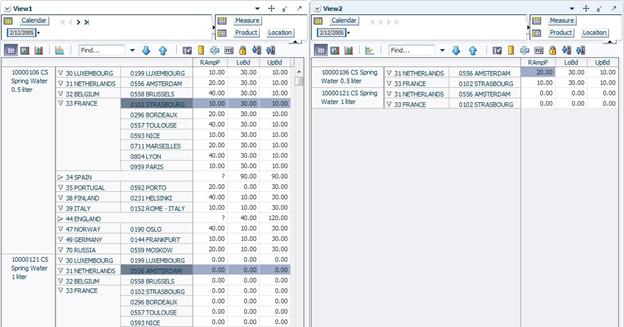
In the above example, a position filter has been applied to View 2. This results in a single position, 33 France. If you now goes to View 1 and uses the page edge controls to scroll through the available locations, view 2 cannot synchronize because it only has a single location dimension. This situation will persist until more locations are made visible when another position filter is applied (or the show and hide option is used).
Position filtering also updates charts. Where positions are hidden by the position filter, the graph is updated to reflect the changed data. In the example below, the pie chart is currently showing data for all stores in the district of France.
A position filter is then applied. As a result, the district of France is filtered so that only three stores are visible. The pie chart is updated accordingly.
If a different position filter is applied, the chart will update accordingly. In the final example, the position filter has been reapplied, and as a result, the data from the Spain district is visible. The chart now shows the pertinent stores from Spain.
Other RPAS functionality can affect the use of position filters.
Position filtering only operates on visible measures. In addition, if the measures are hidden when the filter is applied, they will remain hidden after the filter has been applied. In order to see which measures are hidden, double click any dimension tile in the page edge. This brings up the Dimension dialog box. The Show and Hide tab shows which measures are visible and which are hidden.
If you hides positions with the position filter applied, the position filter will remain in effect. If you show additional positions, the position filter will be overridden.
If you opt to view batch alerts, the current position filter will be removed. Batch alerts can be selected for viewing from the opening page or from the View menu if a workbook is currently open.
Once a workbook has been opened to show batch alerts, the alerts can be filtered using position filtering.
After the batch alerts have been displayed, you can reapply the position filter.
Once applied, position filters can be removed using an option available on the right click menu. This option is not available until a position filter has been applied.
When workbooks are copied or saved with position filtering applied, the following applies: