| Program Performance Analysis Tools |
| Program Performance Analysis Tools |
| C H A P T E R 5 |
|
The Performance Analyzer Graphical User Interface |
The Performance Analyzer analyzes the program performance data that is collected by the Sampling Collector. This chapter provides a brief description of the Performance Analyzer GUI, its capabilities, and how to use it. The online help system of the Performance Analyzer provides information on new features, the GUI displays, how to use the GUI, interpreting performance data, finding performance problems, troubleshooting, a quick reference, keyboard shortcuts and mnemonics, and a tutorial.
This chapter covers the following topics.
For an introduction to the Performance Analyzer in tutorial format, see .
For a more detailed description of how the Performance Analyzer analyzes data and relates it to program structure, see Chapter 7.
To start the Performance Analyzer from the command line, use the analyzer(1) command. The syntax of the analyzer command is as follows:
% analyzer [-h] [-j jvm-path] [-J jvm-options] [-V] [-v] [experiment-list] |
Here, experiment-list is a list of experiment names or experiment group names. See for information on experiment names. If you omit the experiment name, the Open Experiment dialog box is displayed when the Performance Analyzer starts. If you give more than one experiment name, the data for all experiments are added in the Performance Analyzer.
The options for the analyzer command are described in TABLE 5-1.
To exit the Performance Analyzer, choose File  Exit.
Exit.
For information on starting the Performance Analyzer from the IDE, see the Program Performance Analysis Tools Readme, which is available through the documentation index at file:/opt/SUNWspro/docs/index.html. If the Sun ONE Studio 8, software is not installed in the /opt directory, ask your system administrator for the equivalent path on your system.
The Performance Analyzer window contains a menu bar, a tool bar, and a split pane for data display. Each pane of the split pane contains several tab panes that are used for the displays of the Performance Analyzer. The Performance Analyzer window is shown in FIGURE 5-1.
The menu bar contains a File menu, a View menu, a Timeline menu and a Help menu. In the center of the menu bar, the selected function or load object is displayed in a text box. This function or load object can be selected from any of the tabs that display information for functions. From the File menu you can open new Performance Analyzer windows that use the same experiment data. From each window, whether new or the original, you can close the window or close all windows.
The toolbar contains a number of buttons grouped according to menu.
The first group contains buttons related to the File menu: 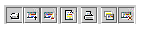
The second group contains buttons related to the View menu: 
The third group contains buttons related to the Timeline menu: 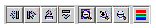
Additionally, the toolbar contains a Find text box, with buttons to Find Previous and Find Next. 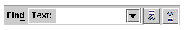 Find text box, find previous and find next buttons.
The following subsections describe what is displayed in each of the tabs.
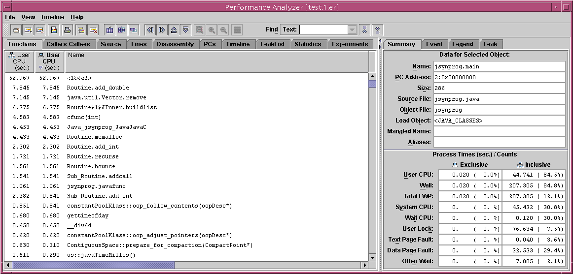
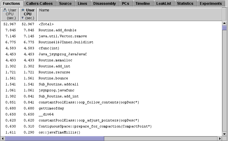
The Functions tab shows a list of functions and load objects and their metrics. Only the functions that have non-zero metrics are listed. The term functions includes Fortran functions and subroutines, C functions, C++ functions and methods, and Java methods. The function list in the Java representation shows metrics against the interpreted Java methods, and any native methods called. The Expert-Java representation additionally lists methods that were dynamically compiled by the HotSpot virtual machine. In the machine representation, multiple HotSpot compilations of a given method will be shown as completely independent functions, although the functions will all have the same name. All functions from the JVM will be shown as such.
The Functions tab can display inclusive metrics and exclusive metrics. The metrics initially shown are based on the data collected and on the default settings. The function list is sorted by the data in one of the columns. This allows you to easily identify which functions have high metric values. The sort column header text is displayed in bold face and a triangle appears in the lower left corner of the column header. Changing the sort metric in the Functions tab changes the sort metric in the Callers-Callees tab unless the sort metric in the Callers-Callees tab is an attributed metric.
 [ D ]
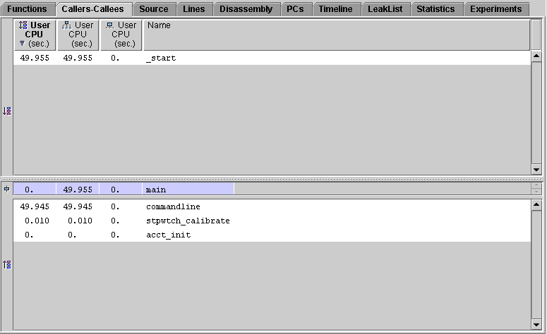
[ D ]The Callers-Callees tab shows the selected function in a pane in the center, with callers of that function in a pane above it, and callees of that function in a pane below it. Functions that appear in the Functions tab can appear in the Callers-Callees tab.
In addition to showing exclusive and inclusive metric values for each function, the tab also shows attributed metrics. If either an inclusive or an exclusive metric is shown, the corresponding attributed metric is also shown. The default metrics shown are derived from the metrics shown in the Function List display.
The percentages given for attributed metrics are the percentages that the attributed metrics contribute to the selected function's inclusive metric. For exclusive and inclusive metrics, the percentages are percentages of the total program metrics.
You can navigate through the structure of your program, searching for high metric values, by selecting a function from the callers or the callees pane. Whenever a new function is selected in any tab, the Callers-Callees tab is updated to center it on the selected function.
The callers list and the callees list are sorted by the data in one of the columns. This allows you to easily identify which functions have high metric values. The sort column header text is displayed in bold face. Changing the sort metric in the Callers-Callees tab changes the sort metric in the Functions tab.
In the machine representation for applications written in the Java programming language, the caller-callee relationships will show all overhead frames, and all frames representing the transitions between interpreted, compiled, and native methods.
 [ D ]
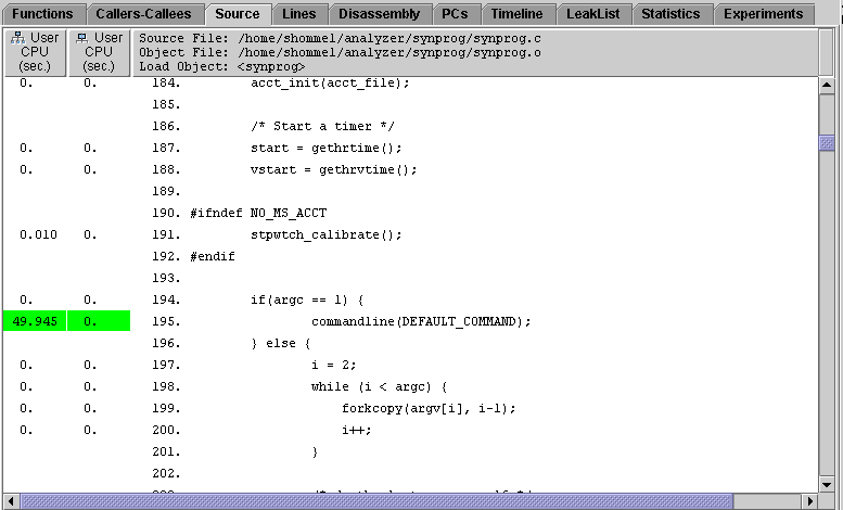
[ D ]The Source tab shows the source file that contains the selected function. Each line in the source file for which instructions have been generated is annotated with performance metrics. If compiler commentary is available, it appears above the source line to which it refers.
Lines with high metric values have the metrics highlighted. A high metric value is one that exceeds a threshold percentage of the maximum value of that metric on any line in the file. The entry point for the function you selected is also highlighted.
The choice of performance metrics, compiler commentary and highlighting threshold can be changed in the Set Data Presentation dialog box. The default choices can be set in a defaults file. See Default-Setting Commands for more information on setting defaults.
You can view annotated source code for a C or C++ function that was dynamically compiled if you provide information on the function using the collector API, but you only see non-zero metrics for the selected function, even if there are more functions in the source file.
The source for a Java method corresponds to the source code in the .java file from which it was compiled, with metrics on each source line. In the machine representation, the source from compiled methods will be shown against the Java source; the data will represent the specific instance of the compiled-method selected.
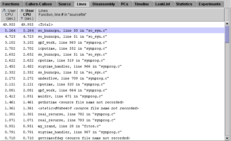
The Lines tab shows a list of source lines and their metrics. The source lines are represented by the function name followed by the line number and the source file name.
The source lines are ordered by the data in one of the columns. This allows you to easily identify which lines have high metric values. The sort column header text is displayed in bold face and a triangle appears in the lower left corner of the column header. You can select the sort metric column by clicking its column header.
If you select a source line, this line becomes the selected object, and is displayed in the Selected Object text box. When you click the Source tab, the source code from which the line came is displayed with the source line selected. When you click the Functions tab or Callers-Callees tab, the function from which the line came is the selected function.
The Disassembly tab shows a disassembly listing for the object file that contains the selected function, annotated with performance metrics for each instruction. The instructions can also be displayed in hexadecimal. Instructions that are marked with an asterisk are synthetic instructions. These instructions are generated for hardware counters that count memory access events if the search for the PC that triggered the event is unsuccessful.
If the compilation object was compiled with debugging information, and the source code is available, it is inserted into the listing. Each source line is placed above the first instruction that it generates. Source lines can appear in blocks when compiler optimizations of the code rearrange the order of the instructions. If compiler commentary is available it is inserted with the source code. The source code can also be annotated with performance metrics.
If the compilation object was compiled with support for hardware counter profiling (see ) control transfer targets are distinguished from the (immediately following) instruction at the (same) address with the label "<branch target>" and by marking their address with an asterisk. Hardware counter events corresponding to memory operations which were collected with backtracking enabled (see and ) may be associated with these synthetic instructions whenever they prevent the causal instruction from being determined.
If the compilation object was compiled with both debugging information and support for hardware counter profiling, memory referencing instructions may be annotated with the referenced dataobject descriptor, which constitutes the basis for program data-oriented analyses (see The Data Objects Tab).
Lines with high metric values have the metric highlighted. A high metric value is one that exceeds a threshold percentage of the maximum value of that metric on any line in the file.
If the selected function was dynamically compiled, you only see instructions for that function. If you provided information on the function using the Collector API (see ), you only see non-zero source metrics for the specified function, even if there are more functions in the source file. You can see instructions for Java compiled methods without using the Collector API. The disassembly of any Java method shows the bytecode generated for it, with metrics against each bytecode, and interleaved Java source, where available. In the machine representation, disassembly for compiled methods will show the generated machine assembler code, not the Java bytecode.
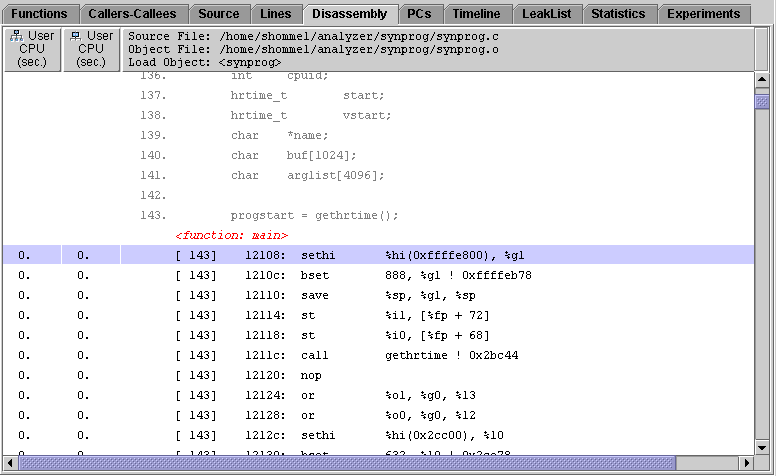
The choice of performance metrics, compiler commentary, highlighting threshold, source annotation and hexadecimal display can be changed in the Set Data Presentation dialog box. The default choices can be set in a defaults file. See Default-Setting Commands for more information on setting defaults.
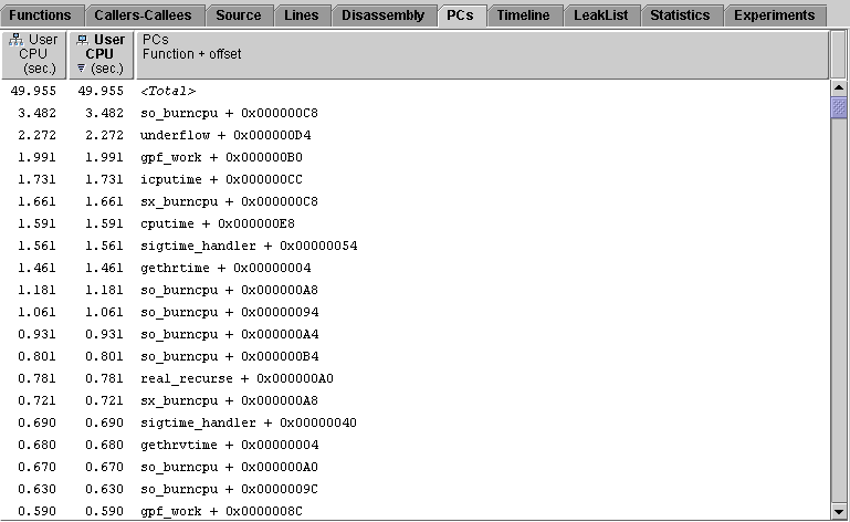
The PCs tab shows a list of program counter addresses and the metrics for the corresponding instructions. The PCs are represented by the function name and the offset relative to the start of the function.
For hardware counter experiments profiling events corresponding to memory operations which were collected with backtracking enabled (see and ), a PC may have been adjusted to that of the most likely memory-referencing instruction, or backtracking may have been blocked, e.g., by an intervening control transfer target. Where backtracking is blocked, a synthetic PC is created to distinguish it from the actual instruction PC: such synthetic PCs are visibly distinguished with an appended asterisk character (e.g., "main + 0x0000ABC4*" represents the synthetic control transfer target with the same address as the instruction "main + 0x0000ABC4").
The list of PCs is ordered by the data in one of the columns. This allows you to easily identify which PCs have high metric values. The sort column header text is displayed in bold face and a triangle appears in the lower left corner of the column header. You can select the sort metric column by clicking its column header.
If you select a PC from the list this PC becomes the selected object. When you click the Disassembly tab, the disassembly listing for the function from which the PC came is displayed with the PC selected. When you click the Source tab, the source listing for the function from which the PC came is displayed with the line containing the PC selected. When you click the Functions tab or Callers-Callees tab, the function from which the PC came is the selected function.
The choice of performance metrics and sort metric can be changed in the Set Data Presentation dialog box. The default choices can be set in a defaults file. See Default-Setting Commands for more information on setting defaults.
For applications written in the Java programming language, a PC for a method (in the Java representation) corresponds to the method-id and a bytecode index into that method; a PC for a native function corresponds to a machine PC. The callstack for a Java thread may have a mixture of Java PCs and machine PCs. It will not have any frames corresponding to Java housekeeping code, which does not have a Java representation.
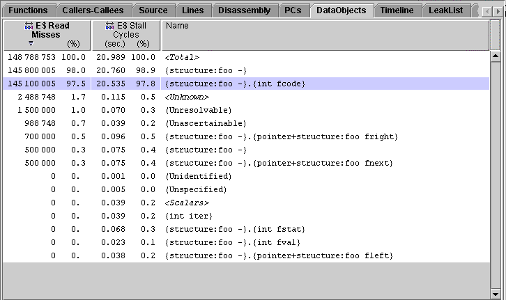
The Data Objects tab is only presented when Data Space Display Mode has been enabled (see The Formats Tab and datamode { on| off }). The Data Objects tab shows a list of dataobjects and their metrics. Only dataobjects that have non-zero metrics are listed. The term "dataobjects" includes program constants, variables, arrays and aggregates such as structures and unions, along with distinct aggregate elements. Various synthetic dataobjects are also defined as required (see The <Unknown> Dataobject).
The Data Objects tab shows only data-derived metrics from hardware counter events for memory operations collected with backtracking enabled for compilation objects built with associated hardware profiling support. The metrics initially shown are based on the data collected and the data presentation settings for inclusive and exclusive (code) metrics. The dataobject list is sorted by the data in one of the columns. This allows you to easily identify which dataobjects have high metric values. The sort column header text is displayed in bold face and a triangle appears in the lower left corner of the column header. The initial sort metric is based on the corresponding inclusive or exclusive (code) metric, if a data-derived metric variant is appropriate.
Data-derived metrics apply only to dataobjects, and are similar to inclusive (code) metrics: the metric value for an element of an aggregate is also included in the metric value for the aggregate.
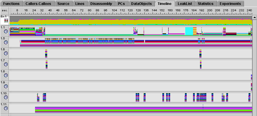
The Timeline tab shows a chart of events as a function of time. The event and sample data for each experiment and each LWP (or thread or CPU) is displayed separately, rather than being aggregated. The Timeline display allows you to examine individual events recorded by the Collector.
Data is displayed in horizontal bars. The display for each experiment consists of a number of bars. By default, the top bar shows sample information, and is followed by a set of bars for each LWP, one bar for each data type (clock-based profiling, hardware counter profiling, synchronization tracing, heap tracing), showing the events recorded. The bar label for each data type contains an icon that identifies the data type and a number in the format n.m that identifies the experiment (n) and the LWP (m). LWPs that are created in multithreaded programs to execute system threads are not displayed in the Timeline tab, but their numbering is included in the LWP index. See Parallel Execution and Compiler-Generated Body Functions for more information. You can choose to display data for threads or for CPUs (if recorded in an experiment) rather than for LWPs, using the Timeline Options dialog box. The index m is then the index of the thread or the CPU.
The sample bar shows a color-coded representation of the process times, which are aggregated in the same way as the timing metrics. Each sample is represented by a rectangle, colored according to the proportion of time spent in each microstate. Clicking a sample displays the data for that sample in the Event tab. When you click a sample, the Legend and Summary tabs are dimmed.
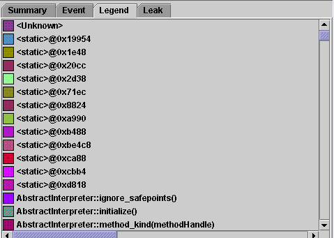
The event markers in the other bars consist of a color-coded representation of part of the call stack. Each function in the call stack is represented by a small colored rectangle. These rectangles are aligned vertically. By default, the leaf function is at the top. The call stack can be aligned on the leaf function or the root function using the Timeline Options dialog box. The color coding of the functions in the call stack is displayed in the Legend tab and can be changed using the Timeline Color Chooser dialog box.
Selecting a sample bar or event marker results in the corresponding horizontal data channel being highlighted, along with a vertical cursor showing the duration of the sample or event. This will be a line, 1 pixel wide, if the event is instantaneous or of short duration.
Clicking a colored rectangle in an event marker selects the corresponding function and PC from the call stack and displays the data for that event and that function in the Event tab. The selected function is highlighted in both the Event tab and the Legend tab and the PC address for the event is displayed in the menu bar as a function with an offset from the function. Clicking the Disassembly tab displays the annotated disassembly code for the function with the line for the PC selected.
 [ D ]
[ D ]
The Event tab is displayed by default in the right pane when the Timeline tab is selected. The Legend tab, also in the right pane, shows color-coding information for functions.
The default choice of data type, display type (by LWP, CPU or thread), call stack alignment and maximum depth can be set in a defaults file. See Default-Setting Commands for more information on setting defaults.
In the Java representation, each Java thread's event callstack is shown with its Java methods. In the machine representation, the timeline will show bars for all threads LWPs or CPUs, and the callstack in each will be the machine-representation callstack.
The LeakList tab shows all leak and allocation events that occurred in the program. The tab is divided into two panels: a top panel, showing leak events, and a bottom panel, showing allocation events. Timeline information appears at the top of the tab, and call stacks for the events appear in both panels.
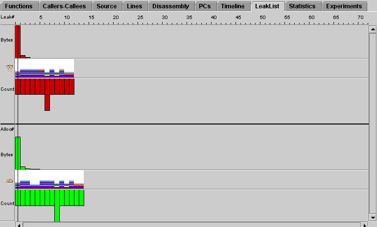
The leak and allocation event panels are each subdivided into three sections: the number of bytes leaked/allocated, the call stack for the selected event, and the number of times the leak or allocation has occurred. To select an individual leak or allocation event, single-click on any data portion of the display. Data for the selected event will be displayed in the Leak tab on the right side of the main analyzer display. Pressing the arrow buttons in the toolbar will step event selection back and forth between the displayed events in each bar. The up and down buttons are disabled because, unlike on the timeline, there is no correlation between leaks and allocations.
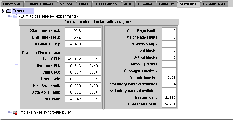
The Statistics tab shows totals for various system statistics summed over the selected experiments and samples, followed by the statistics for the selected samples of each experiment. The process times are summed over the microaccounting states in the same way that metrics are summed. See for more information.
The statistics displayed in the Statistics tab should in general match the timing metrics displayed for the <Total> function in the Functions tab. The values displayed in the Statistics tab are more accurate than the microstate accounting values for <Total>. But in addition, the values displayed in the Statistics tab include other contributions that account for the difference between the timing metric values for <Total> and the timing values in the Statistics tab. These contributions come from the following sources:
For information on the definitions and meanings of the execution statistics that are presented, see the getrusage(3C) and proc(4) man pages.
The Experiments tab is divided into two panes.
The top pane contains a tree that shows information on the experiments collected and on the load objects accessed by the collection target. The information includes any error messages or warning messages generated during the processing of the experiment or the load objects. Experiments that were incomplete but otherwise readable by the Analyzer have a cross in a red circle superimposed on the experiment icon.
The bottom pane lists error and warning messages from the Performance Analyzer session.
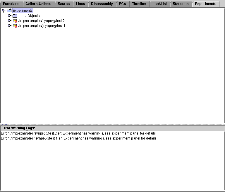
Data in the Experiments tab is organized into a hierarchical tree, with "Experiments" shown as its root node. Beneath that is the "Load Objects" branch node, with additional nodes representing each currently loaded experiment. When expanded, the "Load Objects" node will list all loadobjects in the experiments, with any errors or warnings recorded at the time of archiving, and a message about the process that did the archiving. In addition, if "-A copy" was specified to collect, or the "collector archive copy" command was given to dbx, or the "-A" flag was given during an explicit invocation of er_archive, a copy of each load object (the a.out and any shared objects referenced) will be copied into the archive subdirectory. Expanding an experiment node reveals information about how the experiment was collected, such as the target command, collector version, host name, data collection parameters, and warning messages.
Each experiment has an archive subdirectory, which contains binary files describing each loadobject referenced in the loadobjects file. These files are produced by er_archive, which runs at the end of data collection. If the process terminates abnormally, er_archive may not be invoked, in which case, the archive files are written by er_print or Analyzer when first invoked on the experiment.
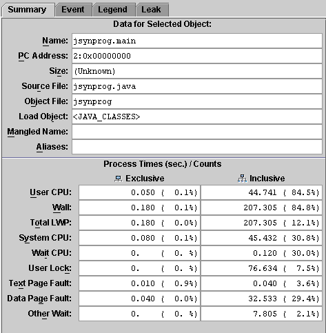
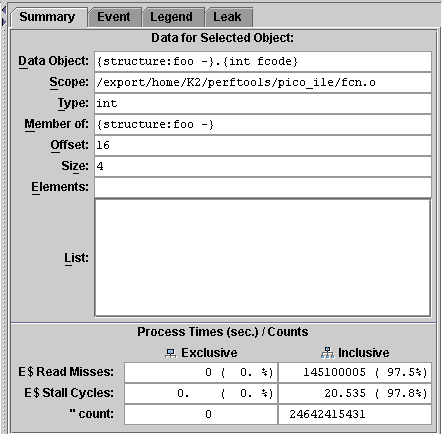
The upper section of the Summary tab shows information about the selected object. When the selected object is a loadobject, a function, a source line or a PC, the information displayed includes the name, address and size, and for functions, source lines and PCs, the name of the source file, object file and load object. Selected functions are shown with their mangled names and also any aliases which may have been defined. In Dataspace Display mode (see The Formats Tab and datamode { on| off }), the alias for a selected PC is its descriptor (when it is ascertainable from the available debugging information). When the selected object is a dataobject, the information displayed includes the name, scope, type and size. If the selected dataobject is an aggregate (such as a structure or union), a list is shown with its elements and their sizes and offsets in the aggregate. If the selected dataobject is a member of an aggregate, the aggregate's name is shown along with the member's offset in the aggregate.
The lower section of the Summary tab shows all the available metrics for the selected object. For loadobjects, functions, source lines and PCs, both exclusive and inclusive metrics are shown as values and percentages, with an additional line for hardware counters that count in cycles. For dataobjects, only data-derived metrics are shown.
The information in the Summary tab is not affected by metric selection. The Summary tab is updated whenever a new object is selected.
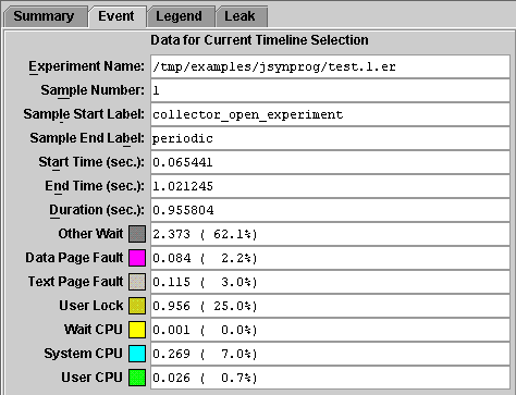
The Event tab shows the available data for the selected event, including the experiment name, event type, leaf function, timestamp, LWP ID, thread ID, CPU ID, Duration, and Micro State information. Below the data panel the call stack is displayed with the color coding that is used in the event markers for each function in the stack. Clicking a function in the call stack makes it the selected function.
For hardware counter events corresponding to memory operations which were collected with backtracking enabled (see and ), corresponding data address information is also shown where determinable and verifiable.
When a sample is selected, the Event tab shows the sample number, the start and end time of the sample, and a list of timing metrics. For each timing metric the amount of time spent and the color coding is shown. The timing information in a sample is more accurate than the timing information recorded in clock profiling.
The Legend tab shows the mapping of colors to functions for the display of events in the Timeline tab. The Legend tab is only enabled when an event is selected in the Timeline tab. It is dimmed when a sample is selected in the Timeline tab. The color coding can be changed using the color chooser in the Timeline menu.
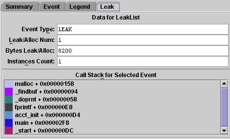
The leak tab shows detailed data for the selected leak or allocation in the LeakList tab. It is divided into two panels: a top panel, showing data for the LeakList, and a bottom panel, showing the call stack for the selected event.
The top panel displays the event type, leak/allocation number, number of bytes leaked or allocated, and the instances count. In the bottom panel, clicking on a function in the call stack makes it the selected function.
This section describes some of the capabilities of the Performance Analyzer and how its displays can be configured.
The Performance Analyzer computes a single set of performance metrics for the data that is loaded. The data can come from a single experiment, from a predefined experiment group or from several experiments.
To compare two selections of metrics from the same set, you can open a new Analyzer window by choosing File Open New Window from the menu bar. To dismiss this window, choose File Close from the menu bar in the new window.
To compute and display more than one set of metrics--if you want to compare two experiments, for example--you must start an instance of the Performance Analyzer for each set.
The Performance Analyzer allows you to compute metrics for a single experiment, from a predefined experiment group or from several experiments. This section tells you how to load, add and drop experiments from the Performance Analyzer.
Opening an Experiment. Opening an experiment clears all experiment data from the Performance Analyzer and reads in a new set of data. (It has no effect on the experiments as stored on disk.)
Adding an Experiment. Adding an experiment to the Performance Analyzer reads a set of data into a new storage location in the Performance Analyzer and recomputes all the metrics. The data for each experiment is stored separately, but the metrics displayed are the combined metrics for all experiments. This capability is useful when you have to record data for the same program in separate runs--for example, if you want timing data and hardware counter data for the same program.
To examine the data collected from an MPI run, open one experiment in the Performance Analyzer, then add the others, so you can see the data for all the MPI processes in aggregate. If you have defined an experiment group, loading the experiment group has the same effect.
Dropping an Experiment. Dropping an experiment clears the data for that experiment from the Performance Analyzer, and recomputes the metrics. (It has no effect on the experiment files.)
If you have loaded an experiment group, you can only drop individual experiments, not the whole group.
Once you have experiment data loaded into the Performance Analyzer, there are various ways for you to select what is displayed.
You can open the Set Data Presentation dialog box using the following toolbar button, or by selecting View->Set Data Presentation... from the menu.

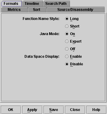
The Set Data Presentation dialog contains the following individual tabs: Metrics, Sort, Source/Disassembly, Formats, Timeline, and Search Path.
You can select the metrics that are displayed and the sort metric using the Metrics and Sort tabs of the Set Data Presentation dialog box. The choice of metrics applies to all tabs. The Callers-Callees tab adds attributed metrics for any metric that is chosen for display.
All metrics are available as either a time in seconds or a count, and as a percentage of the total program metric. Hardware counter metrics for which the count is in cycles are available as a time, a count, and a percentage.
The Sort tab allows you to set the sort metric and order in which the metric columns are displayed. To change the sort metric, double-click the metric or its radio button. To change the order of the metrics, click the metric then use the Move Up or Move Down buttons to move the metric.
The sort tab allows the data to be sorted by any of the following:
The visible metrics appear in bold text.
You can select the threshold for highlighting high metric values, select the classes of compiler commentary and choose whether to display metrics on annotated source code and whether to display the hexadecimal code for the instructions in the annotated disassembly listing from the Source/Disassembly tab of the Set Data Presentation dialog box.
The formats tab allows you to specify whether you want C++ function names to be displayed in short or long form. The long form is the full, demangled name including parameters; the short form does not include the parameters. The formats tab also allows you to set the Java representation (to on, expert, or off), and lets you enable or disable the data space display.
You can choose to display event data for LWPs, for threads or for CPUs in the Timeline tab, choose the number of levels of the call stack to display, choose the alignment of the call stacks in the event markers, and select the data types to display.
Sets the path used for finding source, object etc. files. The search path is also used to locate the .jar files for the Java Runtime Environment (JRE) on your system. The special directory name $expts refers to the set of current experiments, in the order in which they were loaded. To change the search order, single-click on an entry and press the Move Up/Move Down buttons. The compiled-in full pathname will be used if a file is not found in searching the current path setting.
Filtering by Experiment, Sample, Thread, LWP and CPU. You can control the information in the Performance Analyzer displays by specifying only certain experiments, samples, threads, LWPs, and CPUs for which to display metrics. You make the selection using the Filter Data dialog box. Selection by thread, by sample, and by CPU does not apply to the Timeline display.
You can open the Filter Data dialog box using the following toolbar button:
Showing and Hiding Functions. For each load object, you can choose whether to show metrics for each function separately or to show metrics for the load object as a whole, using the Show/Hide Functions dialog box. You can open the Show/Hide Functions dialog box using the following toolbar button, or by selecting View->Show/Hide Functions... from the menu.
The settings for all the data displays are initially determined by a defaults file, which you can edit to set your own defaults.
The default metrics are read from a defaults file. In the absence of any user defaults files, the system defaults file is read. A defaults file can be stored in a user's home directory, where it will be read each time the Performance Analyzer is started, or in any other directory, where it will be read when the Performance Analyzer is started from that directory. The user defaults files, which must be named .er.rc, can contain selected er_print commands. See Default-Setting Commands for more details. The selection of metrics to be displayed, the order of the metrics and the sort metric can be specified in the defaults file. The following table summarizes the system default settings for metrics.
For each function or load-object metric displayed, the system defaults select a value in seconds or in counts, depending on the metric. The lines of the display are sorted by the first metric in the default list.
For C++ programs, you can display the long or the short form of a function name. The default is long. This choice can also be set up in the defaults file.
You can save any settings you make in the Set Data Presentation dialog box in a defaults file.
See Default-Setting Commands for more information about defaults files and the commands that you can use in them.
Find tool. The Performance Analyzer includes a Find tool in the toolbar that you can use to locate text in the Name column of the Functions tab and the Callers-Callees tab, and in the code column of the Source tab and the Disassembly tab. You can also use the Find tool to locate a high metric value in the Source tab and the Disassembly tab. High metric values are highlighted if they exceed a given threshold of the maximum value in a source file. See Selecting the Data to Be Displayed for information on selecting the highlighting threshold.
Using the performance data from an experiment, the Performance Analyzer can generate a mapfile that you can use with the static linker (ld) to create an executable with a smaller working-set size, more effective instruction cache behavior, or both. The mapfile provides the linker with an order in which it loads the functions.
To create the mapfile, you must compile your program with the -g option or the -xF option. Both of these options ensure that the required symbol table information is inserted into the object files.
The order of the functions in the mapfile is determined by the metric sort order. If you want to use a particular metric to order the functions, you must collect the corresponding performance data. Choose the metric carefully: the default metric is not always the best choice, and if you record heap tracing data, the default metric is likely to be a very poor choice.
To use the mapfile to reorder your program, you must ensure that your program is compiled using the -xF option, which causes the compiler to generate functions that can be relocated independently, and link your program with the -M option.
| Program Performance Analysis Tools | 817-0922-10 |
Copyright © 2003, Sun Microsystems, Inc. All rights reserved.

