| Analyzing Program Performance with Sun WorkShop |
Sampling Collector Reference
This chapter introduces the Sampling Collector and explains how to use it. It covers the following topics:
- What the Sampling Collector Collects
- Collecting Performance Data in Sun WorkShop
- Starting a Process Under the Collector in dbx
- Attaching to a Running Process
- Using the Collector for Programs Written with MPI
The Sampling Collector collects performance data from your target application and the kernel under which your application is running, and writes that data to an experiment record file. An experiment is the data collected during one execution of your application.
Unless you have specified otherwise, experiment-record files generated by the Sampling Collector have the extension
.n.er, where n is an integer 1 or higher. The default experiment-file name istest.n.er. If you use the filename.1.erformat for your experiment-record file name, the Collector automatically increments the names of subsequent experiments by one--for example,my_test.1.eris followed bymy_test.2.er,my_test.3.er, and so on.
Caution – Do not use thermutility to delete an experiment-record file. The actual experiment information is stored in a hidden directory,.filename.n.er, whichrmdoes not remove. To delete an experiment record file and also its hidden directory, use the performance-tool utilityer_rm, which is included with the Collector and Analyzer. See theer_rmman page for information about usinger_rm.
What the Sampling Collector Collects
The Sampling Collector records performance data, and organizes the data into samples, each of which represents an interval within an experiment. The Sampling Collector terminates one sample and begins a new one in the following circumstances:
- When it encounters a breakpoint (see Introduction to Sun WorkShop for information about setting breakpoints in Sun WorkShop Debugging)
- When the sampling interval expires, if you have set a sampling interval
- When you choose Collect
New Sample or click the New Sample button, if you have selected manual sampling
The data recorded for each sample consists of microstate accounting information from the kernel and various other statistics maintained within the kernel.
All data recorded at sample points is global to the program and does not include function-level metrics. However, if function-level metrics have been recorded during the sampling interval, the Collector associates these function metrics with the sampling interval during which they were collected.
The Sampling Collector can gather the following types of function-level information:
- Clock-based profiling data
- Thread-synchronization wait tracing
- Hardware-counter overflow profiling
Exclusive, Inclusive, and Attributed Metrics
The Collector collects exclusive, inclusive, and attributed function and load-object metrics.
- Exclusive data applies to time spent in the function itself.
- Inclusive data applies to time spent in the function itself and also to time spent in any function it calls. Time from callees is counted only for calls from the given function.
- Attributed data of a given function applies to the sum of metrics that occur in a callee of the given function and any functions the callee calls as a result of the call from the given function. The following conditions apply to attributed metrics:
- The attributed metric for any caller of a given function is the metric that occurs in the given function and any function or functions it calls as a result of the caller's call to it.
- A caller's attributed metric equals the contribution of the given function to the caller's inclusive metric.
- The sum of the attributed metrics of all a given function's callers equals the given function's inclusive metric.
- The attributed metric of a callee of the given function is that fraction of the callee's inclusive metric that resulted from the call from the given function.
- The difference between a callee's attributed metric and its inclusive metric represents that portion of the callee's inclusive metric that resulted from calls from callers other than the given function.
- The inclusive metric of the given function equals its own exclusive metric plus the sum of all the attributed metrics of the given function's callees.
Clock-Based Profiling Data
Clock-based profiling records information to support the following metrics:
- User CPU time. Time during which your application is running on the CPU.
- Total LWP time. Total execution time across all LWPs (lightweight processes).
- Wall-clock time. LWP time spent in thread 1.
- System CPU time. Total CPU time, within the operating system or in trap state for the LWP.
- System wait time. LWP time spent waiting for the CPU, for a lock, or for a kernel page, or time spent sleeping or stopped.
- Text-page fault time. LWP time spent waiting for a text page.
- Data-page fault time. LWP time spent waiting for a data page.
This information appears in the Function List display and the Callers-Callees window of the Analyzer. (See Examining Metrics for Functions and Load-Objects.) It also appears in the Summary Metrics window and annotated source and disassembly.
Note – For multiprocessor experiments, times other than wall-clock time are summed across all LWPs in the process. Total time equals the wall-clock time multiplied by the average number of LWPs in the process. Each record contains a timestamp and the IDs of the thread and LWP running at the time of the clock tick.
Clock-based profiling helps answer the following kinds of questions:
- How much of the available resources does the application consume?
- Which functions are consuming the most resources?
- Which source lines and disassembly instructions consume the most resources?
- How did the program arrive at this point in the execution?
Thread Synchronization Wait Tracing
In multithreaded programs, thread synchronization wait tracing keeps track of wait time on calls to thread-synchronization routines in the threads library; if the real-time delay exceeds a certain user-defined threshold, an event is recorded for the call, as well as the wait time, in seconds.
Each record contains a timestamp and the IDs of the thread and LWP running at the time of the clock stamp. Synchronization-delay information supports the following metrics:
- Synchronization-delay events. The number of calls to a synchronization routine where the wait exceeded the prescribed threshold.
- Synchronization wait time. Total of wait times that exceeded the prescribed threshold.
This information appears in the Function List display and the Caller-Callee window of the Sampling Analyzer (see Examining Metrics for Functions and Load-Objects). It also appears in the Summary Metrics window and annotated source and disassembly.
Hardware-Counter Overflow Profiling
Hardware-counter overflow profiling records the callstack of each LWP at the time a designated hardware counter of the CPU on which the LWP is running overflows. The data recorded includes a timestamp and the IDs of the thread and the LWP.
The Collector allows you to select the type of counter whose overflow is to be monitored, and to set an overflow value for it. Typically, counters keep track of such things as instruction-cache misses, data-cache misses, cycles, or instructions issued or executed.
Note – Hardware-counter overflow profiling can be done only on Solaris 8 for SPARC (UltraSPARC III) machines and on x86 (Pentium II and compatible products). On other machines, this feature is disabled.
Hardware-counter overflow profiling produces data to support count metrics.
Global Information
Global information about your program includes the following kinds of data:
- Execution statistics. Include page fault and I/O data, context switches, and a variety of page residency (working-set and paging) statistics. This information appears in the Execution Statistics display of the Sampling Analyzer. (See Examining Execution Statistics.)
- Address-space data (optional). Consists of page-referenced and page-modified information for every segment of the application's address space. This information appears in the Address Space display of the Sampling Analyzer. (See Examining Address-Space Information.)
Collecting Performance Data in Sun WorkShop
Before you can collect data, you must do the following:
- Load your program into the Debugging window. (See Introduction to Sun WorkShop for information about how to start Sun WorkShop and access the Debugging window.)
- Ensure that run-time checking is turned off (the default).
Collecting data requires two steps:
- Specifying the kinds of data you want to collect and where you want to store the data.
- Running the Collector.
To specify the kinds of data you want to collect:
1. From the WorkShop window menu bar, choose Window
- The WorkShop Sampling Collector window appears.
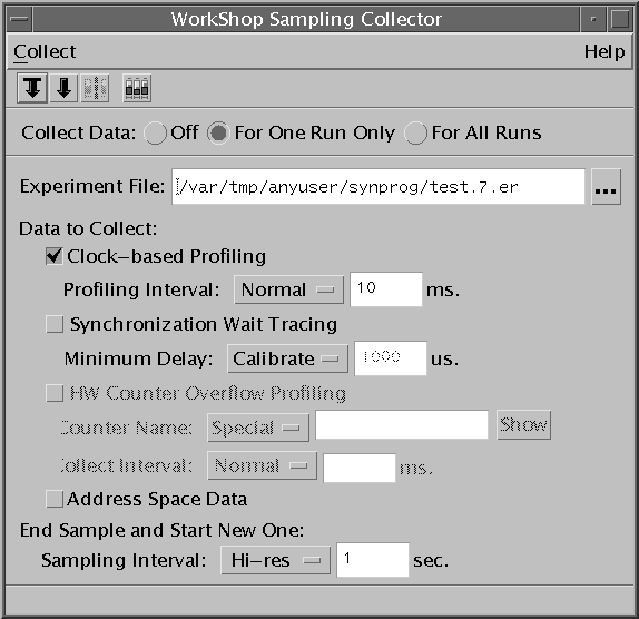
FIGURE 3-1 The Sampling Collector Window2. Use the Collect Data radio buttons to specify whether you want to collect data for this one run only or for multiple runs.
- If you select "for one run only", the Collector is disabled after your program has run once and the data for that run is stored in the experiment record file.
- If you select "for all runs", the Collector remains active after your program has finished running, and for each subsequent run, it creates a new experiment record file to store the data for that run.
- If you select "off", the Collector is disabled and collects and stores no data until you select one of the other Collect Data radio buttons.
3. In the Experiment File text box, specify the path and file name of the experiment-record file in which you want the data to be stored.
- The default experiment-record file name provided by the Collector is
test.1.er. If you want to name your file a different file name, you must enter a path (if you do not want it to be stored in the default directory) and file name for it.- If you use the
.1.ersuffix for your experiment-record file name, the Sampling Collector automatically increments the names of subsequent experiments by one. For example,test.1.eris followed bytest.2.er.4. To collect clock-based profiling information, ensure that the Clock-Based Profiling Data check box is selected. (This check box is selected by default.)
- You can accept the Normal profiling interval (10 milliseconds) or from the Profiling Interval list box you can select Hi-res (1 millisecond) or Custom, where you set your own interval in milliseconds.
- High-resolution profiles record ten times as much data as normal profiles for any given run. To support high-resolution profiling, the operating system must be running with a high-resolution clock routine. You can specify a high-resolution routine by adding the following line to the file
/etc/system, and then rebooting:
Note – If you try to set high-resolution profiling on a machine whose operating system does not support it, the Collector posts a warning message and reverts to the highest resolution supported. A custom setting that is not a multiple of the resolution supported by the system is rounded to the nearest multiple of that resolution, and the Collector issues a warning message.
5. To collect information about thread-synchronization wait counts and times, select the Synchronization Wait Tracing check box.
- To specify the threshold beyond which tracing begins:
- You can accept the default, Calibrate (the threshold is determined at run time).
- From the Minimum Delay list box you can select a threshold of:
6. To collect information about hardware counter overflows, select the HW Counter Overflow Profiling check box.7. Choose a category of counters from the Counter Name menu, then click Show for a list of all counters available in that category. The user-recognizable name of the counter you select appears in the Counter Name text box.8. To specify the number of increments that take place between one overflow event and the next, choose the default Normal from the Collect Interval menu (the value of Normal depends on the counter you have selected), or choose Custom and type a value in the Collect Interval text box.
Note – All hardware counters are platform dependent, so the list of available counters differs from system to system. Some systems do not support hardware-counter overflow profiling. On such systems, this option is disabled.
9. To collect information about memory allocation in the address space, select the Address Space Data check box.10. You can accept the default Hi-res sampling interval (a 1-second interval), or from the Sampling Interval list box you can select Normal (a 10-second interval), Custom (set your own interval in seconds), or Manual, in which you signal the end of the current sample and the beginning of a new one by either choosing Collect
Now you are ready to collect data. To run the Sampling Collector, in the WorkShop Sampling Collector window:
- Choose File

Starting a Process Under the Collector in
dbxYou can run the Collector from
dbx, as well as from the Sun WorkShop Debugging window. To do this:1. Start your program indbxby typing:
dbxprogram_name2. Press the space bar until the(dbx)prompt appears.3. Use thecollectorcommand with its various arguments to collect data and generate an experiment record:
collectorargument
- The
collectorcommand arguments are listed in TABLE 3-1.
To get a listing of available
collectorcommand arguments, type the following at the(dbx)prompt and press Enter:
help collectorAttaching to a Running Process
The Collector allows you to attach to a running process and collect performance data from the process.
If you want to collect thread synchronization wait tracing, load the library
libcollector.sobefore you start the executable, so the Collector's wrapper around the real synchronization routines is referenced, rather than the actual routines themselves. If you are collecting only profiling data or hardware-counter overflow profiling, you do not need to preload the collector library, although you can do so if you wish.
- Set the environment variable
LD_PRELOADto point tolibcollector.so, as shown in TABLE 3-2.
- install_directory is the directory that contains your distribution (normally, it is
/opt/).
Note – Remove theLD_PRELOADsetting after the run, so it will not remain in effect for all other programs started from the same shell.
To attach to the executable and collect data:
1. Start the executable.2. Determine the executable's PID, and attachdbxto it.
3. Enable data collection:
- Start collecting data, either directly in
dbxusing thecollectorcommand, or from the Sampling Collector window.- Use the
contcommand to resume the target process fromdbx.
Note – If you have started the executable fromdbxwithout enabling data collection, you can pause the target fromdbxand then execute the preceding instructions to start data collection during the run.
Using the Collector for Programs Written with MPI
The Collector can collect performance data from multi-process programs that use the Sun Message Passing Interface (MPI), if you use the Sun Cluster Runtime Environment (CRE) command
mprunto launch the parallel jobs. Use ClusterTools 3.1 or a compatible version. See the Sun HPC ClusterTools 3.1 documentation for more information.To collect data from MPI jobs, you must either start the MPI processes under
dbx, or attachdbxto each process separately. For example, suppose you run MPI jobs using a command line like the following:
mprun -np 2 a.out[program-arguments]You can replace that command line with the following:
mprun -np 2 dbx a.out < collection.scriptwhere
collection.scriptis adbxscript, described in the following paragraphs.When this example is executed, two MPI processes from the executable
a.outrun, and two experiments are created, namedtest.M.erand test.N.er, where M and N are the PIDs of the two MPI processes.Your file
collection.scriptmust ensure that the experiments created are uniquely named. Otherwise, because thedbxinstances that generate the experiments are being run simultaneously, two or more of thedbxinstances might attempt to create experiments with the same name. One way to ensure uniquely named files is to make your script specify that eachdbxinstance must use a file name with the process ID of the MPI process in it:
You can also create experiments named with the MPI rank, by using a slightly different
dbxscript in which you stop the target program immediately following a call to MPI_Comm_rank() and use the rank to specify the experiment directory. For example, suppose your MPI program contains one of the following statements on line 17:
- For a C program:
- For a Fortran program:
Change
collection.scriptto read as follows:
With this modification,
mpruncreates experiments named with the rank of the MPI process to which they correspond.To examine the data collected from the MPI processes, open one experiment in the Analyzer, then add the others, so you can see the data for all the MPI processes in aggregate. See Starting the Analyzer and Loading an Experiment and Adding Experiments to the Analyzer for more information.
You can also use
er_printto print out the data.er_printaccepts multiple experiments on the command line. For information about usinger_print, see Chapter 5.
|
Sun Microsystems, Inc. Copyright information. All rights reserved. Feedback |
Library | Contents | Previous | Next | Index |