18 Working with Forecast Consumption
This chapter includes the following topics:
18.1 About Forecast Consumption
Forecast consumption logic takes into account forecasts and total customer sales including shipments when planning, and uses whichever is greater to calculate requirements within user defined periods. Open sales orders and shipments "consume" the forecast until sales quantities exceed forecast quantities, at which point, the excess sales order demand drives requirements planning.
18.2 Setting Up Forecast Consumption
In order to use forecast consumption, you must set up the following:
-
Add planning fence information in the Item/Branch Plant
-
Set up User Defined Codes (UDCs)
-
Set Up a Customer/Item Relationship
-
Define forecast consumption periods
-
Set up for planning generation
-
Set up Time Series
18.2.1 Adding Planning Fence Information
From Inventory Management (G41), choose Inventory Master/Transactions
From Inventory Master/Transactions (G4111), choose Item Branch/Plant Information
To enter planning fence information in the Item Branch/Plant
On Item Branch/Plant Information
Figure 18-1 Item Branch/Plant Information screen
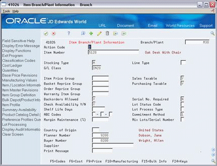
Description of ''Figure 18-1 Item Branch/Plant Information screen''
-
Choose Manufacturing (F10) to display the Plant Manufacturing Data - Branch screen.
Figure 18-2 Plant Manufacturing Data screen
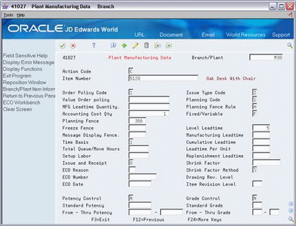
Description of ''Figure 18-2 Plant Manufacturing Data screen''
-
Enter H in the following field:
-
Planning Fence Rule
-
-
Enter the number of days greater than or equal to the planning horizon in the following field:
-
Planning Fence
For example, with planning horizon periods set for 12 monthly buckets, set Planning Fence field to at least 366.
-
18.2.2 Setting Up UDCs
From (G00), choose General User Defined Codes
All sales order document types in the inclusion rules that you specify in planning program processing options need to be in UDC 40/CF if you are using forecast consumption. When you ship confirm an order, and the document type is set up in this UDC, the system stores the quantity in the Forecast Shipment Summary file (F3462) and these quantities continue to consume forecast in the appropriate period (-SHIP appears on the time series) until their scheduled pick date is prior to the current forecast consumption period.
|
Note: If a sales order document type is added to 40/CF after shipments are made for orders with that doc type, the orders already shipped will not be included in F3462, and therefore the -SHIP for the period in which they were shipped will not appear. |
The following illustrates setting up the UDC 40/CF.
On General User Defined Codes
Figure 18-3 General User Defined Codes (Add Sales Order Document) screen
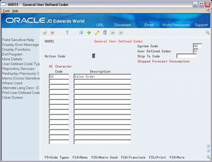
Description of ''Figure 18-3 General User Defined Codes (Add Sales Order Document) screen''
-
On General User Defined Codes, enter 40 in the System Code field
-
Enter CF in the User Defined Codes field.
-
Review or change the following fields, as needed:
-
Code
-
Description
-
-
Click Add.
18.2.3 Setting Up a Customer/Item Relationship
Each sales order includes two address book numbers, sold to and ship to, and you must define which number the system uses to match a sales order to a forecast. You specify the default address number in the Forecast Consumption by Customer processing option in the Master Planning Schedule (P3482) program.
You can use the Forecast Consumption Customer Address Relationship program (P3406) to establish exceptions to the default you set up. The system stores this information in the Customer Address Relationship Revisions file (F3406). You can set up the relationship for the customer only, or you can set it up for a combination of item and customer.
To set up customer item relationship
From Material Planning (G34), Enter 29
From Material Planning Setup (G3440), choose Requirements Planning Setup
From Material Planning Setup (G3442), choose Customer/Item Relationship
Figure 18-4 Customer/Address Relationship screen
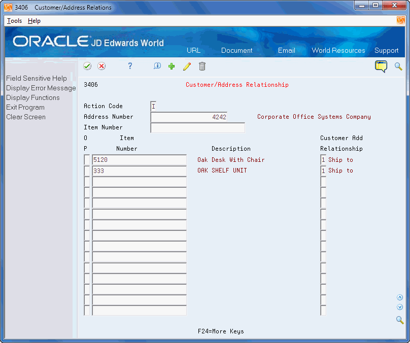
Description of ''Figure 18-4 Customer/Address Relationship screen''
-
On Customer/Item Relationship, complete one of the following fields:
-
Address Number
-
Item Number
-
-
Complete the following fields and click Add.
-
Item Number
-
Customer Address Relationship
-
| Field | Explanation |
|---|---|
| Customer Address Relationship | This determines whether a ship-to or sold-to address of a sales order is used to consume customer specific forecast. |
18.2.4 Defining Monthly Forecast Consumption Periods
In order to use forecast consumption, forecast consumption periods must be defined. These periods determine what forecasts are consumed by what sales orders, depending on where forecasts and sales orders fall within the specified periods.
There are two valid Period Types:
-
FC - Forecast consumption period
-
TS - Time series bucket
The end date of each forecast consumption period is defined with FC in the Period Type field. When you enter forecast consumption periods, this information will apply system wide, can be any length, and can end on any date. If the end date entered is a non-workday, the system will use the last workday prior as the end date. The beginning date of a period is the first working day after the prior period end date.
Each period end date forces a time series bucket. When you run Planning Generation, the daily and weekly buckets specified in the planning horizon processing options will appear on the time series, but the months specified will be replaced by forecast consumption periods. The TS period type is used to generate time series buckets when forecast consumption periods are greater than a month.
For example, if quarterly forecast consumption periods are set up without any TS periods, only quarterly time series buckets will be written after any daily and/or weekly buckets. If time series buckets within the forecast consumption periods (i.e. monthly time series buckets within quarterly forecast consumption periods) are required, they are defined by the TS period type.
From Material Planning (G34), choose Hidden Selection 29
From Material Planning Setup (G3440), choose Requirements Planning Setup
From Material Planning Setup (G3442), choose Forecast Consumption Periods
To define monthly forecast consumption periods
On Forecast Consumption Periods
-
Complete the following field for each consumption period to add:
-
Period End Date
-
-
To set up a monthly forecast consumption period, enter FC in the following field:
-
Period Type
Figure 18-5 Forecast Consumption Periods screen
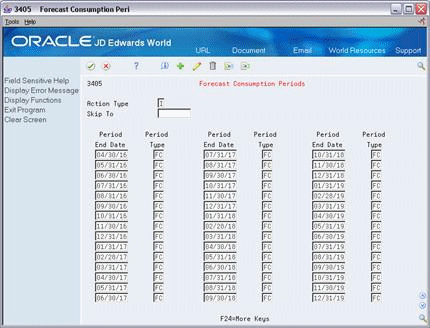
Description of ''Figure 18-5 Forecast Consumption Periods screen''
-
-
If the forecast consumption periods are greater than a month, you can generate time series buckets in between period end dates. Enter TS in the following field:
-
Period Type
-
Figure 18-6 Forecast Consumption Period (Time Series Buckets) screen

Description of ''Figure 18-6 Forecast Consumption Period (Time Series Buckets) screen''
18.2.5 Setting Up for Planning Generation
You must set the processing options for P3482 or Master Planning Schedule - Multiple Plant (P3483) to activate forecast consumption logic and select two past due periods.
Two past due periods are only appropriate in conjunction with forecast consumption logic. The reason two past due buckets are used for forecast consumption is because there are times when the current forecast consumption period will cross over the generation date, leaving part of the period in the past. The Past Due 1 bucket includes supply and demand quantities due prior to the beginning of the current forecast consumption period. The Past Due 2 bucket consists of the period from the beginning date of the current forecast consumption period to the generation date of the planning run. Unlike other planning fence rules, forecasts prior to the generation date are still relevant (within the current forecast consumption period).
See Section 54.1, "Master Planning Schedule - Plant Maintenance (P3482)."
See Section 54.4, "Multi-Facility - Gross Regeneration (P3483)."
18.3 Working with Forecast Consumption by Customer
Forecast Consumption by Customer enhances your ability as a supplier to meet the requirements from large customers. When dealing with large customers, you might want to consider the demand for each customer separately and plan production quantities accordingly. You can set up the system to net forecasts and sales orders for a particular customer separately, so that you can plan more accurately for the specific demand coming from individual customers.
When you create your production or distribution plan, you enter a forecast for a specific customer and the system considers the customer forecast and customer demand. Because the forecast record includes a value in the Customer Number field, the system can search for sales orders with matching customer numbers in the ship-to or sold-to field to calculate the remaining demand for the customer. You specify whether the system uses the value in the ship-to or sold-to field from the sales order by defining a customer address relationship.
Whether your use the P3482 or P3483, you create a version and set the Forecast Type, Forecast Consumption, and the Forecast Consumption by Customer processing options to calculate the forecast consumption by customer. Additionally, for P3483, you must:
-
Set the Interplant Demand processing option to consume the forecast.
-
Ensure that the items have a planning fence rule of C, G or H.
When you run P3482, you can apply forecast consumption logic to individual customers. MRP reads the forecast and sales orders and applies forecast consumption logic for every customer to calculate actual daily demand. Customer-specific forecasts are consumed by only sales orders for the same customer. The system stores the demand in the Forecast file (F3460) as a new forecast type. The system derives the final daily demand for the item by accumulating daily demands from individual customers. Additionally, MRP uses this forecast type as a solo source of independent demand.
This forecast consumption logic applies to items that have the planning fence rule of G, C or H. The system compares the forecast to sales within time series buckets, as defined by planning horizon settings, for items with planning fence rule C or G. The system compares sales and shipments within established forecast consumption periods for items with a rule of H.
The system uses the following process:
-
Check the Item Branch record for the item to for a time fence rule of C, G or H.
-
Examine the Forecast File table (F3460) and the Sales Order Header File table (F4201) record for each customer.
-
Compare sales orders and the forecast for each customer to determine which is greater.
The system stores the greater value of the two in the F3460 as a new forecast record with a forecast type that indicates that it is the result of a Forecast Consumption by Customer calculation.
When there is a customer-specific forecast in the entire planning period, sales orders consume the customer specific forecast even if there is no forecast in the period. For example, when there is a sales order for 04/16/18 and there is no forecast for the same customer in the period, the sales order consumes the customer-specific forecast if there is a forecast for the same customer on another day.
Following is an example of Forecast Consumption by Customer Planning using fence rule G:
| Date | 4/1 | 4/2 | 4/3 | 4/4 | |
|---|---|---|---|---|---|
| Forecast | Generic
4242 |
100
10 |
100
10 |
100 | 100 |
| Sales Order | 4343
4242 |
80
8 |
105
11 |
80
10 |
111
10 |
| Greater of Forecast or Sales Order | Generic
4242 |
100
10 |
105
11 |
100
10 |
111
10 |
| Total Adjusted Demand | 110 | 116 | 110 | 121 |
In this example, there is no forecast for 4242 on 04/03, but the system processes the data as if there is a forecast for a quantity of zero on that day, and a sales order for 4242 does not consume the generic forecast.
When you set the Forecast Type for MPS processing option, existing forecasts that have the same forecast type as the one you specify in the processing option are deleted first.
For time series, unadjusted sales orders, adjusted sales orders, or shipped sales orders do not display. An adjusted forecast includes adjusted sales requirements, and shipped sales orders.
When you run P3483, the system processes the data as it does for P3482, with the following exceptions:
-
In simple consolidation mode, sales orders and forecasts in all branches are treated as if they were in the same branch.
-
When you leave the Interplant Demand to Consume Forecast processing option blank, interplant demand displays as -ID on the time series as it does now.
-
When you enter 1 in the Interplant Demand to Consume Forecast processing option, interplant demand displays as -ID on the time series. However, the quantity is included in the -FCST calculation and -ID displays as a reference.
18.4 Forecast Consumption Example
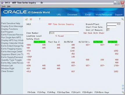
The following sequence of time series demonstrates the use of forecast consumption logic. For these examples, the planning generation processing options specified two weekly buckets then monthly, the forecast consumption periods were monthly, and quantities were forecasted for the first day of the month.
From a generation on the first day of the month, an unadjusted forecast of 1242 (-FCU) appears in the first weekly bucket. The forecast is consumed by 140 that have already shipped (-SHIP), and the sum of the sales orders within the forecast consumption period which is 650 (-SO) for an adjusted forecast quantity of 452 (-FC). The beginning available quantity of 445 minus adjusted forecast and sales order quantities results in an unadjusted ending available of -657 (=EAU) and a planned order for 657 (+PLO).
Figure 18-7 MRP Time Series Inquiry screen
Description of ''Figure 18-7 MRP Time Series Inquiry screen''
Notice that with the forecast consumption processing option behind the time series turned on, period end dates are highlighted making forecast consumption periods easy to see.
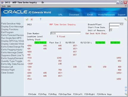
On this time series, generated a few days later, we see the 657 are in process (+WOU/+WO) and another sales order for 100 (-SOU) has been accepted bringing the adjusted sales order quantity to 750 (-SO) and the adjusted forecast to 352 (-FC). Notice that the forecast and shipped quantities now appear in the Past Due 2 bucket; their dates are prior to the generation start date but still within the current forecast consumption period.
Figure 18-8 MRP Time Series Inquiry (Days Later) screen
Description of ''Figure 18-8 MRP Time Series Inquiry (Days Later) screen''
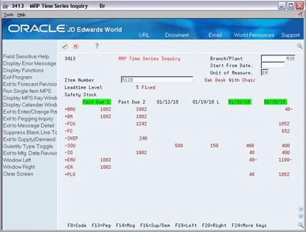
The following week, the work order has been completed, 100 more have shipped, and more sales orders have been accepted (see -SOU of 400 in the 01/31 bucket) to the point that the forecast has been exceeded by 48. The unadjusted forecast of 1242 is fully consumed by the 240 shipped and adjusted sales of 1002; the remaining sales appear in the appropriate bucket (-SO of 48 in the 01/31 bucket) with a planned order for the same quantity as a result.
Figure 18-9 MRP Time Series Inquiry (One Week Later) screen
Description of ''Figure 18-9 MRP Time Series Inquiry (One Week Later) screen''