9 Market Risk - Monte
Carlo Simulation, XVA and PFE
The Market
Risk-Monte Carlo Simulation module enables you to derive counterparty risk
measures and Monte-Carlo Value at Risk (VaR) at the counterparty level and
self-counterparty level. The module enables the application to calculate
counterparty risk, which provides a measure of the
adjustments that should be made to the value of deals, to predict the
possibility of a defaulting counterparty.
Valuation (XVA)
adjustments such as Credit Valuation Adjustment (CVA), Debt Valuation
Adjustment (DVA), Funding Valuation Adjustment (FVA). CVA, DVA, and FVA provide
a single value which can be used as an adjustment to the total value of a set
of positions in a portfolio, considering collateral that can be posted between
the counterparties as determined by the Credit Support Annex (CSA) agreements.
Future exposures
such as Potential Future Exposure (PFE), Expected Positive Exposure EPE,
Expected Negative Exposure (ENE), and Expected Exposure (EE). They provide a measure of the potential loss or gain due to
future market changes and are reported as a table of values for user-specified
future observation dates.
Counterparty risk
values are portfolio-level measures such as values for groups of trades instead
of single quantities for each trade. Future exposures are
computed using American Monte Carlo techniques, for a user-specified
number of Monte Carlo paths and set of future observation dates. To do this, a
global hybrid model must be constructed and used by
all the trades in the simulation. The hybrid model consists of a set of
individual factor models that simulate the dynamics of underlyings of the
selected trades.
The inputs required
to set up a calculation of counterparty risk are:
· Definitions for all the counterparties
and self-counterparties that will be used by the
trades in the calculation.
· Each trade must identify
which counterparty and self-counterparty, netting set and which CSA (that is,
sub-netting set) it is associated with, and be able to identify the list of
underlyings used by that trade.
· Counterparties and self-counterparties
must be organized into the following hierarchy:
§ Parent counterparty: At the top level
of the hierarchy, there is a list of separate counterparty entities. Each
counterparty is considered as a separate entity.
§ Child counterparty (Legal entity):
Within each parent counterparty, there is a list of one or multiple child
counterparties. Each child has a unique name within that parent counterparty.
§ Netting Agreement or Sets: Under each
child counterparty there are one or multiple netting sets. Each netting set has
a unique name within that counterparty, and defines
the level at which all the counterparty risk measures are calculated directly
from the results of netting exposures from different trades, after accounting
for the collaterals. At least one netting set must be defined
for each counterparty.
§ Sub-Netting Agreement or Margin Set or
CSA: At the lowest level of the hierarchy, under each netting set there can be
a set of margin sets. Each margin set has a unique name within that netting set,
and at this level the individual parameters that define the CSA used to
calculate collateral exchange are defined. This allows
you to define separate parameters for subsets of trades that must have
specialized collateral calculation rules, although allowing the net result of
exposures and collateral from those trades to be offset or netted with
exposures from other sets of trades under the same netting set.
§ It is also possible to define a margin
set to consider those trades that are not collateralized.
These trades should be placed in a margin set named Residual.
Topics:
· Navigate
to the Monte Carlo Simulation Summary Window
· Search
for a Business Definition
· Create
and Execute a Business Definition
· Export a
Business Definition
· Approve
or Reject a Business Definition
· Delete a
Business Definition
Navigate to the Monte Carlo Summary window
From the MRMM Home page,
select Market Risk Measurement and Management, click Navigation Menu ![]() ,
select Simulation and then select Monte Carlo Simulation.
,
select Simulation and then select Monte Carlo Simulation.
Figure 55: Monte
Carlo Summary Window
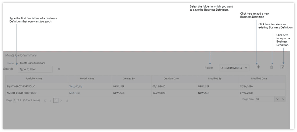
Search for a Business Definition
In the Search
field, type the first few letters of the business definition name that you want
to search. The summaries whose names consist of your search string are displayed in a tabular format.
Figure 56: Monte
Carlo Simulation Summary Window – Search Box
![]()
From the breadcrumb
on top, click the Monte Carlo Summary link to return to the summary window
after viewing details of the business definition.
Page View Options
See the Page View Options section
for details.
Create and Execute a New
Business Definition
A business
definition allows you to set business specific parameters required for
analysis. To define a new Monte Carlo Simulation - business definition, follow
these steps:
1. In the Monte
Carlo Summary window,
click Add
![]() . The
definition window is displayed.
. The
definition window is displayed.
Figure 57: Monte Carlo Simulation Definition Window
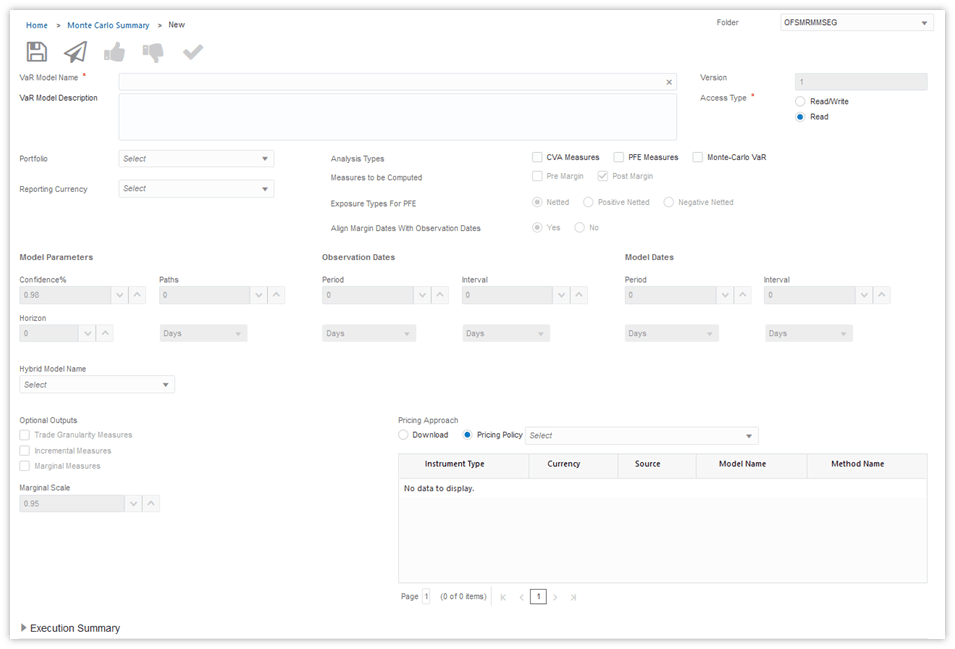
2. Populate the details mentioned in the
following table. Fields marked in red asterisk (*)
are mandatory.
|
Table
29: Monte Carlo Simulation Definition Window – Fields and Descriptions |
|
|
Fields |
Description |
|
VaR Model
Name* |
Enter the
name of the business definition. |
|
VaR Model
Description |
Provide a description of the business
definition. |
|
Version |
Displays the
workflow version of the business definition. |
|
Access Type |
Displays the
access type |
|
Folder |
Select the
folder. |
|
Portfolio* |
Select the
Portfolio from the drop-down list. |
|
Reporting
Currency* |
The currency
in which all the output for a given definition will be
computed. Select the currency code from the drop-down list. |
|
Analysis
Types |
Select the
various computation measures for the business definition. You can select one
or multiple purposes. You can
select both CVA and PFE or Monte Carlo VaR. Each of the subsequent
inputs will be enabled or disabled based on the selected purpose. · CVA Measures · PFE Measures · Monte-Carlo VaR |
|
Measures to be Computed |
Select
pre-margin exposure or post-margin exposures to calculate the counterparty
measures. The default value is Post-Margin. |
|
Exposure
Types for PFE |
Select the
types of exposures to be used for calculating PFE
from the following options: · Netted: It is the sum of pre-margin
or post-margin exposures. · Positive Netted: It is the sum of
positive exposures calculated at the netting set level. · Negative Netted: It is the sum of
negative exposures calculated at the netting set level. |
|
Align Margin
Dates with Observation Dates |
This option enables you to specify whether the Margin (Model)
Dates and Observation Dates should be same. Select Yes or No. If you
select Yes, the Model Date field becomes non-editable. |
|
Model
Parameters |
Specify the
values for the following fields: · Confidence:
Specify the Confidence. Confidence level is required
for PFE calculations. · Paths:
Specify the Number of paths. This is the number of Monte-Carlo paths to be used for the simulations. · Horizon: It
is the time horizon over which the VaR is computed.
This option is available if you select the Analysis
Type as Monte-Carlo VaR. Specify the
horizon in terms of days, months or years. For example, if the horizon is specified as 10 Days then the run will be executed for
VaR outputs with observation date as 10 Days: 10 Days. |
|
Observation
Dates |
Observation
dates are the future dates on which you want to calculate PFE and use for the
exposures to capture the future behavior during CVA computation. Specify the
observation date in Period <Days, Months, Year>: Interval <Days,
Months, Year> format. For example, 30Y:1M, indicates
that one observation date will be generated every month till 30 years. |
|
Model Dates |
Model dates
are additional dates that are used in the simulation
internally, but not used for the final reporting, to obtain better simulation
results and capture more behavior of the deals during their schedules. Specify the
model date in <Period> :< Interval> format. For example, 30Y:30D
which indicates that observation dates are to be
generated, every day for the next 30 years. |
|
Hybrid Model
Name |
The hybrid
model is a set of models to be used for individual
risk factor for generating the paths under Monte Carlo simulation. Select the
strategy from the drop-down menu. See Hybrid Model for
details. |
|
Optional
Outputs |
Specify the
desired optional outputs: · Trade Granularity Measures: Select
this check box to calculate measures at the trade level (in addition to the
counterparty level). This is set to false by default. · Incremental Measures: Select this
check box to calculate incremental measures. This is only available for XVA
and PFE and is set to false by default. · Marginal Measures: Select this check
box to calculate marginal measures. This is only available for XVA and is set
to false by default. |
|
Marginal
Scale |
The scaling
value used for marginal XVA calculations. The default value is 0.95. |
|
Pricing
Policy |
It allows
you to select the pricing policy models and methods to be
used for instrument pricing. You can either download or
define the pricing policy. See section Pricing Policy
for details. For the
selected Pricing Policy, the details such as Instrument
Type, Currency, Source, Model Name, Method Name are displayed. |
3. Click Submit ![]() to save and submit
the definition for approval. A confirmation dialog box is
displayed.
to save and submit
the definition for approval. A confirmation dialog box is
displayed.
Or,
Click Save ![]() to
update the definition before submitting it for
approval.
to
update the definition before submitting it for
approval.
4. If you want to execute the business
definition, follow the steps in the Execute
a Business Definition section.
5. Execution Summary
displays the execution history of the business scenarios. Select the execution
to be marked as EOD execution. You can view details of
the execution, such as Execution Date, Execution ID, Execution
Status, and Definition Workflow
Status
in the Execution Summary table.
6. The definition can be
viewed in the Summary window. They are further
used for in the analytics to generate reports.
Execute a Business Definition
To execute a
business definition, follow these steps:
1. Click the business definition name in
the Summary page. The definition window is displayed.
2. Click Edit ![]() .
.
3. Click Execute ![]() to trigger an Ad hoc run. A message
with a date-time editor dialog box is displayed.
to trigger an Ad hoc run. A message
with a date-time editor dialog box is displayed.
4. Specify the date on which the execution
must be performed.
5. If you want to load trade and market
data from stage tables, select Yes in the field Load
Data From Stage Tables,
else select No. Click OK ![]() . The execution is triggered.
. The execution is triggered.
Figure 58: Monte Carlo Simulation Execution - Date-Time Editor
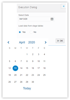
6. Click OK. A confirmation dialog box is displayed.
7. Click OK to confirm.
8. Execution Summary
displays the execution history of the business scenarios. Select the execution
to be marked as EOD execution. You can view details of
the execution, such as Execution Date, Execution ID, Execution
Status, and Definition Workflow
Status
in the Execution Summary table.
Figure 59: Monte
Carlo Simulation Execution Summary

Edit a Business Definition
See the Edit a
Business Definition section for details.
Export a Business
Definition
See the Export a
Business Definition section for details.
Approve or Reject a Business Definition
See the Approve
or Reject a Business Definition section for details.
Delete a Business Definition
See the Delete a
Business Definition section for details.