The Oracle Transfer Pricing Process

This chapter describes the set of steps that you need to follow to transfer price your balance sheet using Oracle Transfer Pricing.

This chapter covers the following topics:

Overview of the Oracle Transfer Pricing Process
Setting Transfer Pricing Rules
Setting Prepayment Rules
Setting and Executing the Transfer Pricing Process Rule
Defining Payment Patterns
Defining Repricing Patterns
Performing Cash Flow Edits
Creating Interest Rate Codes
Accessing Transfer Pricing Detail Cash Flow Results for Audit Purposes
Accessing Transfer Pricing Interest Rate Audit Results
Analyzing Results
Reviewing Processing Errors
Reprocessing Erroneous Accounts
Reconciling the Data

Overview of the Oracle Transfer Pricing Process

Oracle Transfer Pricing (FTP) is based on the Enterprise Performance Foundation (EPF). EPF is the central, integrated data source on which Oracle Financial Services (OFS) applications in Release 12 are built. This description of the Oracle Transfer Pricing process assumes that your system administrator has set up the EPF data repository and has populated it with your enterprise-wide business data.

Important: Oracle Transfer Pricing allows you to transfer price instruments, such as mortgages and commercial loans, stored in the EPF Account tables, also known as Instrument tables, as well as aggregated information, such as cash and other assets, and equity, residing in the Management Ledger table, also known as FEM_BALANCES.

Consequently, while transfer pricing you need to select the Account tables as the data source for instruments and the Management Ledger Table for aggregated information.

The Oracle Transfer Pricing process comprises the following steps:

Important: Although the following list of steps is sequential, not all the users need to follow all the steps. While some of these steps might not be applicable to your product portfolio, some others are optional, and it is up to you to decide whether you want to include them to fine tune your transfer pricing results. All the required steps are explicitly marked as mandatory in the list of steps, as well as in the sections where they are described in detail.

Reconciling the data
Cleansing the data by Performing Cash Flow Edits
Capturing instrument behavior by
- Defining Payment Patterns
- Defining Repricing Patterns
(Mandatory) Deciding on historical rate information and managing it by Creating Interest Rate Codes
Setting Rate Index Rules
(Mandatory) Setting Transfer Pricing Rules
Setting Prepayment Table Rules
Setting Prepayment Rules
Setting Adjustments Rules
Setting Alternate Rate Output Mapping Rules
Creating Propagation Pattern
(Mandatory) Setting and Executing the Transfer Pricing Process Rule
Reviewing processing errors
Accessing Transfer Pricing Detail Cash Flow Results for Audit Purposes
Accessing Transfer Pricing Interest Rate Audit Results
Analyzing results
Reprocessing erroneous accounts

Setting Transfer Pricing Rules

Setting Transfer Pricing rules is one of the mandatory steps in the Oracle Transfer Pricing process. Unless you set Transfer Pricing rules, you cannot transfer price your products. A Transfer Pricing rule is used to manage the association of transfer pricing methodologies to various product-currency combinations. It can also be used to manage certain parameters used in option costing. See: Transfer Pricing Methodologies and Rules.

Setting the Transfer Pricing rules is a two-step process. You need to first create rules and then versions. Transfer pricing methodologies are associated to various product-currency combinations within a version. A Transfer Pricing rule can have more than one version. See: Transfer Pricing Rules.

To reduce the amount of effort required to define the transfer pricing methodologies for various products and currencies, Oracle Transfer Pricing allows you to define transfer pricing methodologies using node level and conditional assumptions.

Node Level Assumptions

Oracle Transfer Pricing uses the Line Item Dimension to represent a financial institution’s product portfolio. Using this dimension, you can organize your product portfolio in a hierarchical structure and define parent-child relationships among different nodes of your product hierarchies. This significantly reduces the amount of work required to define transfer pricing, prepayment, and adjustment methodologies.

You can define transfer pricing, prepayment, and adjustment methodologies at any level of your product hierarchy. Children of parent nodes on a hierarchy automatically inherit the methodologies defined for the parent nodes. However, methodologies directly defined for a child take precedence over those at the parent level. See: Defining Transfer Pricing Methodologies Using Node Level Assumptions.

Conditional Assumptions

This feature allows you to segregate your product portfolio based on common characteristics, such as term to maturity, origination date, and repricing frequency, and assign specific transfer pricing methodologies to each of the groupings.

For example, you can slice a portfolio of commercial loans based on repricing characteristics and assign one global set of transfer pricing, prepayment, and adjustment methods to the fixed-rate loans and another to the floating-rate loans. See: Associating Conditional Assumptions with Transfer Pricing Rules.

Defining Transfer Pricing Methodologies

Transfer Pricing Methodologies and Rules

The transfer pricing methodologies supported by Oracle Transfer Pricing can be grouped into the following two categories:

Cash Flow Transfer Pricing Methods: Cash flow transfer pricing methods are used to transfer price instruments that amortize over time. They generate transfer rates based on the cash flow characteristics of the instruments.

In order to generate cash flows, the system requires a detailed set of transaction-level data attributes, such as, origination date, outstanding balance, contracted rate, and maturity date, which resides only in the Account tables. Consequently, cash flow methods apply only if the data source is Account tables. Data stored in the Management Ledger Tables reflects only accounting entry positions at a particular point in time and do not have the required financial details to generate cash flows, thus preventing you from applying cash flows methodologies to this data.

The cash flow methods are also unique in that Prepayment rules are used only with these methods. You can select the required Prepayment rule when defining a Transfer Pricing Process rule.

See: Setting Prepayment Rules and Cash Flow Calculations, Oracle Financial Services Reference Guide.

Oracle Transfer Pricing supports the following cash flow transfer pricing methods:
Noncash Flow Transfer Pricing Methods: These methods do not require the calculation of cash flows. While some of the noncash flow methods are available only with the Account tables data source, some are available with both the Account and Ledger table data sources.

Oracle Transfer Pricing supports the following noncash flow transfer pricing methods:

Oracle Transfer Pricing also allows Mid-period Repricing. This option allows you to take into account the impact of high market rate volatility while generating transfer prices for your products. However, the mid-period repricing option applies only to adjustable rate instruments and is available only for certain noncash flow transfer pricing methods.

Related Topics

Setting Transfer Pricing Rules

Defining Transfer Pricing Methodologies

Duration

The Duration method uses the MacCauley duration formula:

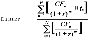
the picture is described in the document text

In this formula:

N = Total number of payments from Start Date until the earlier of repricing or maturity

CFn = Cash flow (such as regular principal, prepayments, and interest) in period n

r = Periodic coupon rate on instrument (current rate/payments per year)

m = Remaining term to cash flow/active payment frequency

tn = Remaining term to cash flow n, expressed in years

Oracle Transfer Pricing derives the MacCauley duration based on the cash flows of an instrument as determined by the characteristics specified in the Account Table and using your specified prepayment rate, if applicable. The duration formula calculates a single term, that is, a point on the yield curve used to transfer price the instrument is being analyzed.

Current rate is defined as current net rate if the processing option Model with Gross Rates is not selected and current gross rate if the option is selected. The current rate is used as the discount rate for each cash flow.
Remaining term to cash flow is the difference between the date of each cash flow and the modeling start date for that instrument.

Defining Transfer Pricing Methodologies

Weighted Term

The Weighted Term method builds on the theoretical concepts of duration. As shown earlier, duration calculates a weighted-average term by weighting each time period, n, with the present value of the cash flow (discounted by the rate on the instrument) in that period.

Since the goal of the Weighted Term method is to calculate a weighted average transfer rate, it weights the transfer rate in each period, yn, by the present value for the cash flow of that period. Furthermore, the transfer rates are weighted by an additional component, time, to account for the length of time over which a transfer rate is applicable. The time component accounts for the relative significance of each strip cash flow to the total transfer pricing interest income/expense. The total transfer pricing interest income/expense on any cash flow is a product of that cash flow, the transfer rate, and the term. Hence, longer term cash flows will have relatively larger impact on the average transfer rate. The Weighted Term method can be summarized by the following formula:

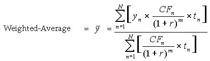
the picture is described in the document text

In this formula:

N = Total number of payments from Start Date until the earlier of repricing or maturity

CFn = Cash flow (such as regular principal, prepayments, and interest) in period n

r = Periodic coupon rate on instrument (current rate/payments per year)

m = Remaining term to cash flow n/active payment frequency

tn = Remaining term to cash flow n, expressed in years

yn = Transfer rate in period n

Defining Transfer Pricing Methodologies

Zero Discount Factors

The Zero Discount Factors (ZDF) method takes into account common market practices in valuing fixed rate amortizing instruments. For example, all Treasury strips are quoted as discount factors. A discount factor represents the amount paid today to receive $1 at maturity date with no intervening cash flows (that is, zero coupon).

The Treasury discount factor for any maturity (as well as all other rates quoted in the market) is always a function of the discount factors with shorter maturities. This ensures that no risk-free arbitrage exists in the market. Based on this concept, one can conclude that the rate quoted for fixed rate amortizing instruments is also a combination of some set of market discount factors. Discounting the monthly cash flows for that instrument (calculated based on the constant instrument rate) by the market discount factors generates the par value of that instrument (otherwise there is arbitrage).

ZDF starts with the assertion that an institution tries to find a funding source that has the same principal repayment factor as the instrument being funded. In essence, the institution strip funds each principal flow using its funding curve (that is, the transfer pricing yield curve). The difference between the interest flows from the instrument and its funding source is the net income from that instrument.

Next, ZDF tries to ensure consistency between the original balance of the instrument and the amount of funding required at origination. Based on the transfer pricing yield used to fund the instrument, the ZDF solves for a single transfer rate that would amortize the funding in two ways:

Its principal flows match those of the instrument.
The Present Value (PV) of the funding cash flows (that is, the original balance) matches the original balance of the instrument.

ZDF uses zero coupon factors (derived from the original transfer rates, see the example below) because they are the appropriate vehicles in strip funding (that is, there are no intermediate cash flows between origination date and the date the particular cash flow is received). The zero coupon yield curve can be universally applied to all kinds of instruments.

This approach yields the following formula to solve for a weighted average transfer rate based on the payment dates derived from the instrument's payment data.

Zero Discount Factors = y =

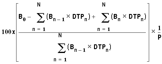
the picture is described in the document text

In this formula:

B0 = Beginning balance at time, 0

Bn-1 = Ending balance in previous period

Bn = Ending balance in current period

DTPn = Discount factor in period n based on the TP yield curve

N = Total number of payments from Start Date until the earlier of repricing or maturity

p = Payments per year based on the payment frequency; (for example, monthly payments gives p=12)

Deriving Zero Coupon Discount Factors: An Example

This table illustrates how to derive zero coupon discount factors from monthly pay transfer pricing rates:

Term in Months	(a) Monthly Pay Transfer Rates	(b) Monthly Transfer Rate: (a)/12	(c) Numerator (Monthly Factor): 1+ (b)	(d) PV of Interest Payments: (b)*Sum((f)/100 to current row	(e) Denominator (1 - PV of Int Pmt): 1 - (d)	(f) Zero Coupon Factor: [(e)/(c) * 100
1	3.400%	0.283%	1.002833	0.000000	1.000000	99.7175
2	3.500%	0.292%	1.002917	0.002908	0.997092	99.4192
3	3.600%	0.300%	1.003000	0.005974	0.994026	99.1053

Defining Transfer Pricing Methodologies

Moving Averages

Under this method, a user definable moving average of any point on the transfer pricing yield curve can be applied to a transaction record to generate transfer prices. For example, you can use a 12-month moving average of the 12-month rate to transfer price a particular product.

The following options become available on the user interface (UI) with this method:

Interest Rate Code: Select the Interest Rate Code to be used as the yield curve to generate transfer rates.
Yield Curve Term: The Yield Curve Term defines the point on the Interest Rate Code that is used.
Historical Term: The Historical Term defines the period over which the average is calculated.

The following table illustrates the difference between the yield curve and historical terms.

Yield and Historical Terms: An Example
Moving Average	Yield Curve Term	Historical Term
Six-month moving average of 1 year rate	1 year (or 12 months)	6 months
Three-month moving average of the 6 month rate	6 months	3 months

The range of dates is based on the effective date minus the historical term plus one, because the historical term includes the effective date. Oracle Transfer Pricing takes the values of the yield curve points that fall within that range and does a straight average on them.

For example, if Effective Date is Nov 21, the Yield Curve Term selected is Daily, and the Historical Term selected is 3 Days, then, the system will calculate the three-day moving average based on the rates for Nov 19, 20, and 21. The same logic applies to monthly or annual yield terms.

Note: The Moving Averages method applies to either data source: Management Ledger Table or Account Tables.

Defining Transfer Pricing Methodologies

Straight Term

When you select the Straight Term method, the system derives the transfer rate using the last repricing date and the next repricing date for adjustable rate instruments, and the origination date and the maturity date for fixed rate instruments.

Standard Calculation Mode:
1. For Fixed Rate Products (Repricing Frequency = 0), use Yield Curve Date = Origination Date, Yield Curve Term = Maturity Date-Origination Date.
2. For Adjustable Rate Products (Repricing Frequency > 0)
  - For loans still in tease period (tease end date > Calendar Period End Date, and tease end date > origination date), use Origination Date and Tease End Date - Origination Date.
  - For loans not in tease period, use Last Repricing Date and Repricing Frequency.
Remaining Term Calculation Mode:
1. For Fixed Rate Products, use Calendar Period End Date and Maturity - Calendar Period End Date.
2. For Adjustable Rate Products, use Calendar Period End Date and Next Repricing Date - Calendar Period End Date.

The following options become available on the application with this method:

Interest Rate Code: Select the Interest Rate Code to be used for transfer pricing the account.
Mid-Period Repricing Option: Select the check box beside this option to invoke the Mid-Period Repricing option.

Note: The Straight Term method applies only to accounts that use Account Tables as the data source.

Defining Transfer Pricing Methodologies

Spread from Interest Rate Code

Under this method, the transfer rate is determined as a fixed spread from any point on an Interest Rate Code. The following options become available on the application with this method:

Interest Rate Code: Select the Interest Rate Code for transfer pricing the account.
Yield Curve Term: The Yield Curve Term defines the point on the Interest Rate Code that will be used to transfer price. If the Interest Rate Code is a single rate, the Yield Curve Term is irrelevant. Select Days, Months, or Years from the drop-down list, and enter the number.
Lag Term: While using a yield curve from an earlier date than the Assignment Date, you need to assign the Lag Term to specify a length of time prior to the Assignment Date.
Rate Spread: The transfer rate is a fixed spread from the rate on the transfer rate yield curve. The Rate Spread field allows you to specify this spread.
Assignment Date: The Assignment Date allows you to choose the date for which the yield curve values are to be picked up. Choices available are the Calendar Period End Date, Last Repricing Date, or Origination Date.
Mid-Period Repricing Option: Select the check box beside this option to invoke the Mid-Period Repricing option.

Note: The Spread From Interest Rate Code method applies to either data source: Management Ledger Table or Account Tables.

Defining Transfer Pricing Methodologies

Spread from Note Rate

To generate transfer prices using this method, you need to provide just one parameter: a rate spread. This spread is added or subtracted from the coupon rate of the underlying transaction to generate the final transfer rate for that record.

While entering the rate spread, make sure to input it with the appropriate positive or negative sign, as illustrated in the following table. The first row describes a situation where you are transfer pricing an asset and want to have a positive matched spread for it (the difference between the contractual rate of the transaction and the transfer rate is positive). Here, you need to enter a negative rate spread.

Example of Rate Spread
Account Type	Matched Spread	Sign of Rate Spread
Asset	Positive (Profitable)	Negative
Asset	Negative (Unprofitable)	Positive
Liability or Equity	Positive (Profitable)	Positive
Liability or Equity	Negative (Unprofitable)	Negative

The following option becomes available on the application when you select this method:

Mid-Period Repricing Option: Select the check box beside this option to invoke the Mid-Period Repricing option.

Note: The Spread From Note Rate method applies only to accounts that use Account Tables as their data source.

Defining Transfer Pricing Methodologies

Redemption Curve

This method allows you to select multiple term points from your transfer pricing yield curve and calculate an average transfer rate based on the weights you assign to each term point. The following options become available on the application with this method:

Interest Rate Code: Select the Interest Rate Code which you want to use as the transfer pricing yield curve.
Assignment Date: The Assignment Date allows you to choose the date for which the yield curve values will be picked up. Choices available are the Calendar Period End Date, Last Repricing Date, or Origination Date.
Percentages/Term Points: See: Defining the Redemption Curve Methodology.
Mid-Period Repricing Option: Select the check box beside this option to invoke the Mid-Period Repricing option.

Note: The Redemption Curve method applies to either data source: Management Ledger Table or Account Tables.

Related Topics

Defining Transfer Pricing Methodologies

Unpriced Account

Under the unpriced account method, the transfer rate for the account is defined as the weighted average of the Line Item dimension members (products). While using the unpriced account methodology, you can specify whether the weighted average of transfer rates has to be taken across all organizational units or for accounts only within that organizational unit.

The following options become available on the application with this method:

Add Dimension Values: Allows you to select the Line Item dimension members (products) whose weighted average transfer rate will be assigned to the product being defined.

Caution: You should not base an unpriced account on another unpriced account, since the processing hierarchy does not properly allow for it.
Across all Organization Units: Allows you to specify whether weighted average of transfer rates has to be taken across all organization units. See: Defining the Unpriced Account Methodology.

Note: The Unpriced Account method applies only to accounts that use Management Ledger Table as their data source.

Related Topics

Defining Transfer Pricing Methodologies

Transfer Pricing Methods and the Mid-Period Repricing Option

The mid-period repricing option allows you to take into account the impact of high market rate volatility while generating transfer rates for your products. However, the mid-period repricing option applies only to adjustable rate instruments and is available only for the following noncash flow transfer pricing methods:

Straight Term.
Spread from Interest Rate Code.
Spread from Note Rate.
Redemption Curve.

The rationale behind mid-period repricing is as follows. If you do not select the Mid-Period Repricing option, Oracle Transfer Pricing computes the transfer rate for an adjustable rate instrument based upon its last repricing date. The assumption behind this method of calculation is that the input transfer rate for a month should be the daily average transfer rate for that entire month. Consequently, all instruments repricing in that month derive their transfer rates from the same (average) transfer pricing yield curve. However, this approach misstates the transfer rate, in periods when the interest rate level has moved substantially since the last repricing.

Take the example of a one-year adjustable rate loan. Suppose it reprices on the 15th of the month, and that transfer rates have moved up 200 basis points since the last reprice. In such a case, the theoretically pure transfer rate for the first half of the month should be 200 basis points lower than the transfer rate for the second half of the month. In order to apply such theoretical accuracy to your transfer pricing results, you should select the Mid-Period Repricing option.

Mid-Period Repricing Computations

The Mid-Period Repricing option uses two columns in the Account Tables (Current- and Prior- Repricing Period Average Daily Balance: CUR_TP_PER_ADB, PRIOR_TP_PER_ADB) that are exclusively devoted to this option. These columns must be accurately populated for the Mid-Period Repricing results to be accurate.

The Mid-Period Repricing Computation process comprises the following steps:

Computation of transfer rate for current repricing period.
If the computed last repricing date > beginning of processing month, roll back to prior repricing date.
Computation of prior period transfer rate.
Repetition of steps 2 and 3 as necessary.
Computation of the final transfer rate by weighting the results (from current and previous repricing periods) by average balances and days.
Application of the final transfer rate to the instrument record.

Typical Calculations

The following diagram depicts a typical Mid-Period Repricing situation where the instrument reprices during the current processing month.

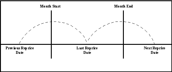
the picture is described in the document text

If an instrument reprices during the current processing month, then there are multiple repricing periods spanning the current month. In this example, there are two repricing periods in the current processing month and the computed last repricing date > beginning of processing month. Consequently, the repricing dates need to be rolled back by the repricing frequency until the Prior Last Repricing Date (Prior LRD) <= Beginning of Month and the Mid-Period Repricing Computation process should be executed as follows:

Computation of transfer rate for current repricing period.

Transfer Pricing Term: Next Reprice Date - Last Reprice Date
Transfer Pricing Date: Last Reprice Date

Number of Days at that Rate: End of Month + 1- Last Reprice Date

Note: If the Computed Next Reprice Date (the next repricing date for a given repricing period) is less than or equal to the End of Month, then the Number of Days calculation uses the Computed Next Reprice Date in place of End of Month. In other words, Number of Days equals the Minimum (End of Month + 1, Computed Next Reprice Date) - Maximum (Beginning of Month, Computed Last Reprice Date).

This example assumes the use of the Straight Term transfer pricing method. The following table describes the logic for the computation of the transfer rates for each method.

Method	Date for Rate Lookup	Terms	Interest Rate Code	Spread
Straight Term	Beginning of Reprice Period	Transfer Pricing Term	Specified in Transfer Pricing rule	Not Applicable
Spread from Interest Rate Code	Beginning of Reprice Period (adjust by Lag Term in TP Rule)	Specified in Transfer Pricing rule	Specified in Transfer Pricing rule	Specified in Transfer Pricing rule
Spread from Note Rate	Beginning of Reprice Period	Transfer Pricing Term	Interest Rate Code from Record	Specified in Transfer Pricing rule
Redemption Curve	Beginning of Reprice Period	Specified in Transfer Pricing rule	Specified in Transfer Pricing rule	Not Applicable

If the computed last repricing date > beginning of processing month, roll back to prior repricing date.

Since the Last Repricing Date is greater than the Beginning of the Processing month, the Roll Back is done as follows:

Computed Next Reprice Date is reset to Last Reprice Date

Computed Last Repricing Date is reset to Last Repricing Date - Reprice Frequency (Prior LRD)
Computation of prior period transfer rate.
- Transfer Pricing Term: Last Reprice Date - Prior LRD
- Transfer Pricing Date: Prior LRD
- Number of Days at that Rate: Last Reprice Date - Beginning of Month
  
  Note: If the Computed Last Reprice Date (the last repricing date for a given repricing period) is greater than the Beginning of Month, then the Number of Days calculation uses Computed Last Reprice Date in place of the Beginning of Month. In other words, Number of Days equals Minimum (End of Month + 1, Computed Next Reprice Date) - Maximum (Beginning of Month, Computed Last Reprice Date).
Repetition of steps 2 and 3 as necessary.

In this example, only one iteration is needed because Prior LRD is less than the Beginning of the Month.
Computation of the final transfer rate by weighting the results (from current and previous repricing periods) by average balances and days.

The calculation makes the following assumptions:
- CUR_TP_PER_ADB is the balance applying since the last reprice date
- PRIOR_TP_PER_ADB is the balance applying to all prior repricing periods
Application of the final transfer rate to the instrument record.

Exceptions to Typical Calculations

There are two exceptions to typical mid-period repricing computations:

Teased Loan Exception

When the TEASER_END_DATE is the first repricing date, it overrides all other values for LAST_REPRICE_DATE and NEXT_REPRICE_DATE. During the Teased Period, then, the Computed Last Repricing Date equals the Origination Date and the Computed Next Reprice Date equals the TEASER_END_DATE. Consequently:

If the TEASER_END_DATE is greater than the CALENDAR_PERIOD_END_DATE, the Mid-Period Repricing does not apply. The logic to compute the Transfer rate is based upon term equal to the TEASER_END_DATE - ORIGINATION_DATE, date equals the ORIGINATION_DATE.
When rolling backwards by repricing frequency, if the TEASER_END_DATE is greater than the Computed Last Repricing Date, Transfer Pricing computes the transfer rates for that period based on the teased loan exception.

Origination Date Exception

While performing mid-period repricing computations, Oracle Transfer Pricing assumes that if the origination date occurs during the processing month, the calculation of the number of days (used for weighting) originates on the first day of the month. This is a safe assumption because the PRIOR_TP_PER_ADB value shows this instrument was not on the books for the entire month. This impact is measured because the PRIOR_TP_PER_ADB value is used in computing the weighted average transfer rate. If Oracle Transfer Pricing were to shorten the number of days (as in the weighted average calculation), it would double-count the impact.

Origination Date Exception: An Example

The following table displays a situation where the origination date occurs during the processing month:

Period 1	Period 2	Period 3
Nov 1 - Nov 10	Nov 11 - Nov 20	Nov 21 - Nov 30
	Loan is originated	Loan reprices
Loan Balance = 0	Loan Balance = 100	Loan Balance = 100
Transfer Rate = 0	Transfer Rate = 6%	Transfer Rate = 8%
Days = 10	Days = 10	Days = 10
Weighting Balance = 50 = PRIOR_TP_PER_ADB	Weighting Balance = 50 = PRIOR_TP_PER_ADB	Weighting Balance = 100 = CUR_TP_PER_ADB

Note: The cumulative average daily balance for period 1 plus period 2 is 50.

Taking the origination date exception into account, the Mid-Period Repricing calculation is done as follows:

(6% * $50 * 20 days) + (8% * $100 * 10 days) / ($50 * 20 days + $100 * 10 days) = 7%

If period 1 was not taken into account, the result would have been, (6% * $50 * 10 days) + (8% * $100 * 10 days) / ($50 * 10 days + $100 * 10 days) = 7.33%, which is incorrect.

Defining Transfer Pricing Methodologies

Defining Transfer Pricing Methodologies Using Node Level Assumptions

In Oracle Transfer Pricing, your product portfolio is represented using the Line Item Dimension. Node Level Assumptions allow you to define transfer pricing, prepayment, and adjustment assumptions at any level of the Line Item (product) dimension. The Line Item dimension supports a hierarchical representation of your chart of accounts, so you can take advantage of the parent-child relationships among different nodes of your product hierarchies while defining transfer pricing, prepayment, and adjustment assumptions. Child nodes for which no assumption has been specified automatically inherit the methodology of their closest parent node.

Node level assumptions can be applied only to the product (Line Item) dimension and not to the currency dimension. Node level assumptions simplify the process of applying rules in the user interface. It is also not required for all rules to assign assumptions to the same nodes. Users may assign assumptions at different levels.

Behavior of Node Level Assumptions

The following graphic displays a sample product hierarchy:

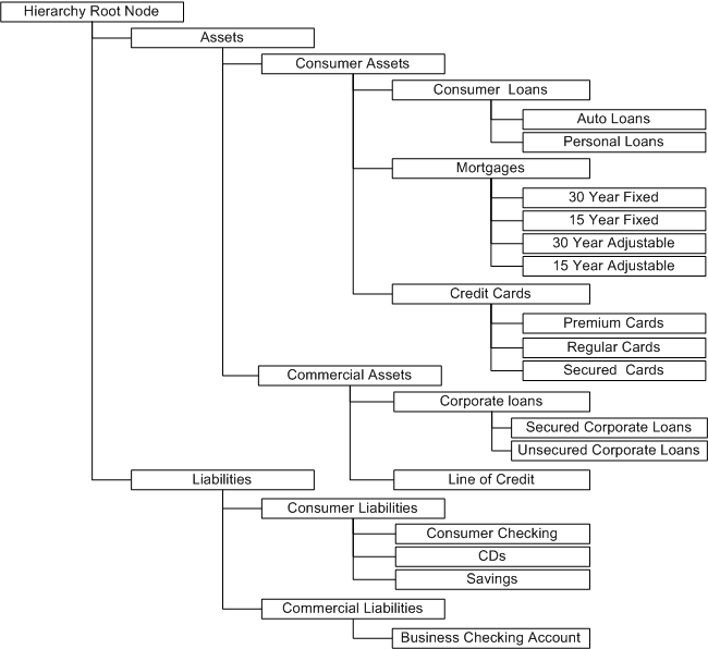
the picture is described in the document text

Suppose you want to transfer price this product hierarchy using the Spread from Interest Rate Code transfer pricing method except for the following products:

Mortgages: You want to transfer price these using the Zero Discount Factors cash flow based method.
Credit Cards: You want to transfer price all but secured credit cards using the Spread from Note Rate method.

To transfer price in this manner, you need to attach transfer pricing methods to the nodes of the product hierarchy as follows:

Hierarchy Root Node: Spread from Interest Rate Code
Mortgages: Zero Discount Factors Cash Flow
Credit Cards: Spread from Note Rate
Secured Credit Cards: Spread from Interest Rate Code

The transfer pricing method for a particular product is determined by searching up the nodes in the hierarchy. Consider the Secured Credit Cards in the above example. Since Spread from IRC is specified at the product level, the system does not need to search any further to calculate the transfer rates for the Secured Credit Cards. However, for a Premium Credit Card the system searches up the hierarchical nodes for the first node that specifies a method. The first node that specifies a method for the Premium Credit Card is the Credit Card node and it is associated with the Spread from Note Rate method.

Note: Not specifying assumptions for a node is not the same as selecting the None methodology (also known as the "Do Not Calculate" method in the Adjustments rule). Child nodes for which no assumptions have been specified automatically inherit the methodology of their closest parent node. So if neither a child node nor its immediate parent has a method assigned, the application searches up the nodes in the hierarchy until it finds a parent node with a method assigned, and uses that method for the child node. However, if no parent node has a method assigned then the application triggers a processing error stating that no assumptions are assigned for the particular product/currency combination. However, if the parent node has the method None assigned to it then the child node inherits None, obviating the need for calculation and for a processing error.

All parameters that are attached to a particular methodology (such as Interest Rate Code) are specified at the same level as the method. If multiple Interest Rate Codes are to be used, depending on the type of the product, the method would need to be specified at a lower level. For instance, if you want to use IRC 211178 for Consumer Products and IRC 3114 for Commercial Products, then the transfer pricing methodologies for these two products need to be specified at the Commercial Products and Consumer Products nodes.

You need not specify prepayment assumptions at the same nodes as transfer pricing methods. For example, each mortgage category can have a different prepayment method while the entire Mortgage node uses the Zero Discount Factors cash flow method for transfer pricing.

Related Topics

Setting Transfer Pricing Rules

Defining Transfer Pricing Methodologies

Associating Conditional Assumptions with Transfer Pricing Rules

Conditional Assumptions

Associating Conditional Assumptions with Transfer Pricing Rules

Oracle Transfer Pricing enhances the setup and maintenance of methodologies by providing conditional logic (optional) to assign transfer pricing, prepayment, and adjustment methods to combinations of products and currencies.

You can define transfer pricing, prepayment, and adjustments methodologies using IF-THEN-ELSE logic based on the underlying characteristics of financial instruments, such as dates, rates, balances, and code values.

In addition, Conditional Assumptions can be attached to any level of the Line Item Dimension hierarchy, allowing assumptions to be inherited from parent nodes to child nodes.

Oracle Transfer Pricing provides a set of user interfaces specially designed to easily build Conditional Assumptions. The logic included in a Conditional Assumption drives the specific Transfer Pricing or Prepayment method that the system would assign to a product-currency combination at run time.

For example, you can use the maturity date column on the commercial loans table to drive the assignment of Transfer Pricing Methods for all the records in that table. You can create one Conditional Assumption to convey the entire Transfer Pricing Methodology logic and attach it to the top-level node of the Line Item Dimension hierarchy representing the commercial loan portfolio. All nodes below the top-level node will inherit the same Transfer Pricing assumptions. See: Overview of Conditional Assumptions.

A Conditional Assumption is made of at least three (IF, THEN, and ELSE) clauses. Each clause is displayed in the user interface as a row. The following table displays a basic Conditional Assumption with three clauses:

Conditional Assumption with Three Clauses
Condition Term	Product Attribute	Operator	Value	TP Method
IF	Repricing Frequency	< >	0
THEN				Cash Flow Weighted Term
ELSE				Straight Term

In the above table, the Cash Flow Weighted Term transfer pricing method is assigned to the designated products that have a repricing frequency not equal to zero. If the repricing frequency is zero, then the Straight Term Transfer Pricing Method is assigned.

Conditional Assumptions can be applied only on detailed accounts (data stored in the Account Tables) and reference only the Cash Flow and Dimension columns that are part of the Account Tables.

Related Topics

Setting Transfer Pricing Rules

Defining Transfer Pricing Methodologies

Availability of Conditional Assumptions

Conditional Assumptions cannot exist independently; they are an extension of Transfer Pricing, Prepayment, and Adjustments Rules.

To define a Conditional Assumption, you need to complete a series of steps beforehand. The following diagram displays, at a high level, how the Conditional Assumptions functionality fits with the overall Create process of a Transfer Pricing rule.

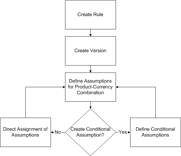
the picture is described in the document text

Assigning Conditional Assumptions is a sub-process within the Create or Update Flow of the Transfer Pricing, Prepayment, and Adjustments rules. Once you create a Rule and a Version, you have two options for defining your transfer pricing methodologies for a product-currency combination.

Direct assignment of a transfer pricing, prepayment, or an adjustment method to a product-currency combination.

This is the conventional method. See: Defining Transfer Pricing Methodologies and Defining Prepayment Methodologies.
Assignment of the methodology through a Conditional Assumption.

In this scenario, you would define IF-THEN-ELSE logic that will determine the Transfer Pricing or Prepayment Methodology for product-currency combinations. See: Conditional Assumptions.

Related Topics

Setting Transfer Pricing Rules

Associating Conditional Assumptions with Transfer Pricing Rules

Defining Transfer Pricing Methodologies Using Node Level Assumptions

Conditional Assumptions

Structure of Conditional Assumptions

A Conditional Assumption comprises blocks of logic. These blocks are in turn built of clauses that exist within each block of logic.

There are three kinds of blocks:

IF
ELSE IF
ELSE

The IF Block

The IF block is always the first of the building blocks in a Conditional Assumption and there can be only one IF block per condition.

The IF block is made of at least two clauses:

The IF clause contains the first logic clause of the block. For a Conditional Assumption, there can be only one IF clause.
The THEN clause is the last clause of the block. You would insert a THEN clause when you have completed the definition of the logic for the block and are ready to assign a Transfer Pricing or Prepayment Method to those records that satisfy the logic.

In addition to the IF and THEN clauses, there are two other clauses you can optionally use to add to the complexity of the IF Block: the AND clause and the OR clause. They are always placed between the IF and the THEN clauses and there is no restriction on the order or amount that you can use.

The ELSE IF Block

The ELSE IF block serves as an alternative to any of the previous logic in a Conditional Assumption. It is used to add new blocks of logic within a Conditional Assumption, thus allowing for definition of more complex logic. There is no limit to the number of ELSE IF blocks you could add to a Conditional Assumption. Besides, their use is optional as the system does not require an ELSE IF block to build a valid Conditional Assumption.

The structure of the ELSE IF block is very similar to the IF block. The first clause indicates the starting point of the logic of the block; the IF and the ELSE IF have the same purpose, except that you can have only one IF clause in an entire Conditional Assumption but unlimited number of ELSE IF clauses. The last clause of the ELSE IF block must also be the THEN clause; it associates the logic of the particular block to a Transfer Pricing or Prepayment Method. Like the IF block, you can have as many AND/OR clauses between the ELSE IF clause and the THEN clause.

The ELSE Block

The ELSE block is the last component of a Conditional Assumption. This block has only one clause. It is used to assign a Transfer Pricing or Prepayment Method to a record of the product-currency combination that does not satisfy the logic defined in all of the previous IF and ELSE IF blocks. The ELSE block ensures that all the records within the product-currency combination defined by you are transfer priced.

Like the IF block there can only be one ELSE block in a Conditional Assumption.

This table illustrates a conditional assumption structure comprising the IF, ELSE IF, and the ELSE blocks.

Conditional Assumption Structure: A Sample
Logic Block	Clause	Account Table Field	Operator	Value	Transfer Pricing Method
IF	IF	Field	Operator	Value
	AND	Field	Operator	Value
	AND	Field	Operator	Value
	OR	Field	Operator	Value
	THEN				Transfer Pricing or Prepayment Method assigned to any instrument that meets logic of the IF Block.
ELSE IF	ELSE IF	Field	Operator	Value
	AND	Field	Operator	Value
	THEN				Transfer Pricing or Prepayment Method assigned to any instrument that meets logic of this ELSE IF Block.
ELSE IF	ELSE IF	Field	Operator	Value
	AND	Field	Operator	Value
	AND	Field	Operator	Value
	OR	Field	Operator	Value
	THEN				Transfer Pricing or Prepayment Method assigned to any instrument that meets logic of this ELSE IF Block.
ELSE	ELSE				Transfer Pricing or Prepayment Method assigned to any instrument that does not meet the logic of any of the previous blocks.

Related Topics

Setting Transfer Pricing Rules

Defining Transfer Pricing Methodologies

Associating Conditional Assumptions with Transfer Pricing Rules

Defining Transfer Pricing Methodologies Using Node Level Assumptions

Conditional Assumptions

Setting Prepayment Rules

One of the major business risks faced by financial institutions engaged in the business of lending is the prepayment risk. Prepayment risk is the possibility that borrowers might choose to repay part or all of their loan obligations before the scheduled due dates. Prepayments can be made by either accelerating principal payments or refinancing.

Prepayments cause the actual cash flows from a loan to a financial institution to be different from the cash flow schedule drawn at the time of loan origination. This difference between the actual and expected cash flows undermines the accuracy of transfer prices generated using cash flow based transfer pricing methods. Consequently, a financial institution needs to predict the prepayment behavior of instruments so that the associated prepayment risk is taken in to account while generating transfer rates. Oracle Transfer Pricing allows you to do this through the Prepayment Rule.

A Prepayment Rule contains methodologies to model the prepayment behavior of various amortizing instruments and quantify the associated prepayment risk. See: Prepayment Methodologies and Rules.

You need to first create rules and then versions. Prepayment methodologies are associated with the product-currency combinations within the versions of the Prepayment rule. See: Prepayment Rules.

Oracle Transfer Pricing allows you to make use of the node level and conditional assumption while defining prepayment methodologies for your products. See: Associating Node Level and Conditional Assumptions with Prepayment Rules.

Important: Prepayment assumptions are used in combination with only the three cash flow based transfer pricing methods: Weighted Term, Duration, and Zero Discount Factors.

Defining Prepayment Methodologies

Prepayment Methodologies and Rules

You can use any of the following three methods in a Prepayment rule to model the prepayment behavior of instruments:

Related Topics

Defining Prepayment Methodologies

Setting Prepayment Rules

Constant Prepayment Method

The Constant Prepayment method calculates the prepayment amount as a flat percentage of the current balance.

You can create your own origination date ranges and assign a particular prepayment rate to all the instruments with origination dates within a particular origination date range.

Note: All prepayment rates should be input as annual amounts.

Related Topics

Prepayment Methodologies and Rules

Defining Prepayment Methodologies

Defining the Constant Prepayment Method

Prepayment Table Method

The Prepayment Table method allows you to define more complex prepayment assumptions compared to the other prepayment methods. Under this method, prepayment assumptions are assigned using a Prepayment table.

You can build a Prepayment table using a combination of up to three prepayment drivers and define prepayment rates for various values of these drivers. Each driver maps to an attribute of the underlying transaction (age/term or rate ) so that the cash flow engine can apply a different prepayment rate based on the specific characteristics of the record.

Note: All prepayment rates should be input as annual amounts.

Prepayment Table Structure

A typical Prepayment table structure includes the following:

Prepayment Drivers: You can build a Prepayment table using one to three prepayment drivers. A driver influences the prepayment behavior of an instrument and is either an instrument characteristic or a measure of interest rates.
The Prepayment Driver Nodes: You can specify one or more node values for each of the prepayment drivers that you select.
Interpolation or Range method: Interpolation or Range methods are used to calculate prepayment rates for the prepayment driver values that do not fall on the defined prepayment driver nodes.

Types of Prepayment Drivers

The prepayment drivers are designed to allow the calculation of prepayment rates at run time depending on the specific characteristics of the instruments for which cash flows are being generated. Although nine prepayment drivers are available, a particular prepayment table can contain only up to three prepayment drivers.

The prepayment drivers can be divided into the following two categories:

Age/Term Drivers: The Age/Term drivers define term and repricing parameters in a Prepayment table. All such prepayment drivers are input in units of months. These Drivers include:
- Original Term: You can vary your prepayment assumptions based on the contractual term of the instrument. For example, you could model faster prepayment speeds for longer term loans, such as a 10-year loan, than for short term loans, such as a 5-year loan. You would then select the Original Term prepayment driver and specify two node values: 60 months and 120 months.
- Repricing Frequency: You can vary your prepayment assumptions based on the repricing nature of the instrument being analyzed. Again, you could specify different prepayment speeds for different repricing frequencies and the system would decide which one to apply at run time on a record by record basis.
- Remaining Term: You can specify prepayment speeds based on the remaining term to maturity. For example, loans with few months to go until maturity tend to experience faster prepayments than loans with longer remaining terms.
- Expired Term: This is similar to the previous driver but instead of looking at the term to maturity, you base your assumptions on the elapsed time. Prepayments show some aging effect such as the loans originated recently experiencing more prepayments than older ones.
- Term to Repricing: You can also define prepayment speeds based on the number of months until the next repricing of the instrument.
Interest Rate Drivers: The Interest Rate drivers allow the forecasted interest rates to drive prepayment behavior to establish the rate-sensitive prepayment runoff. Interest Rate Drivers include:
- Coupon Rate: You can base your prepayment assumptions on the current gross rate on the instrument.
- Market Rate: This driver allows you to specify prepayment speeds based on the market rate prevalent at the time the cash flows occur. This way, you can incorporate your future expectations on the levels of interest rates in the prepayment rate estimation. For example, you can increase prepayment speeds during periods of decreasing rates and decrease prepayments when the rates go up.
- Rate Difference: You can base your prepayments on the spread between the current gross rate and the market rate.
- Rate Ratio: You can also base your prepayments on the ratio of current gross rate to market rate.
  
  The following diagram illustrates a three-driver prepayment table:
  
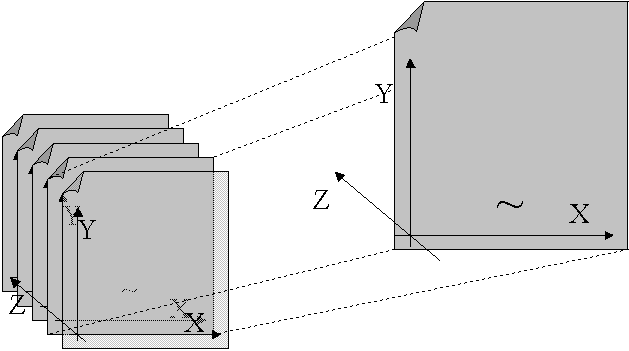
  The ~ signifies a point on the X-Y-Z plane. In this example it is on the second node of the Z-plane. The Z -plane behaves like layers.

Oracle Transfer Pricing allows you to build prepayment tables using the Prepayment Table rule. The Prepayment Table rule can then be referenced by a Prepayment Rule. See: Prepayment Table Rules.

Related Topics

Prepayment Methodologies and Rules

Defining Prepayment Methodologies

Defining the Prepayment Table Rule Method

Arctangent Calculation Method

The Arctangent Calculation method uses the Arctangent mathematical function to describe the relationship between prepayment rates and spreads (coupon rate less market rate).

Note: All prepayment rates should be input as annual amounts.

User defined coefficients adjust this function to generate differently shaped curves. Specifically:

CPRt = k1 - (k2 * ATAN(k3 * (-Ct/Mt + k4)))

where CPRt = annual prepayment rate in period t

Ct = coupon in period t

Mt = market rate in period t

k1 - k4 = user defined coefficients

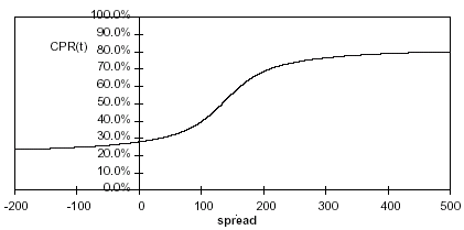
A graphical example of the Arctangent prepayment function is shown below, using the following coefficients:

k1 = 0.3

k2 = 0.2

k3 = 10.0

k4 = 1.2

Each coefficient affects the prepayment curve in a different manner.

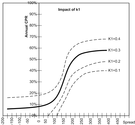
the picture is described in the document text

The following diagram shows the impact of K1 on the prepayment curve. K1 defines the midpoint of the prepayment curve, affecting the absolute level of prepayments. Adjusting the value creates a parallel shift of the curve up or down.

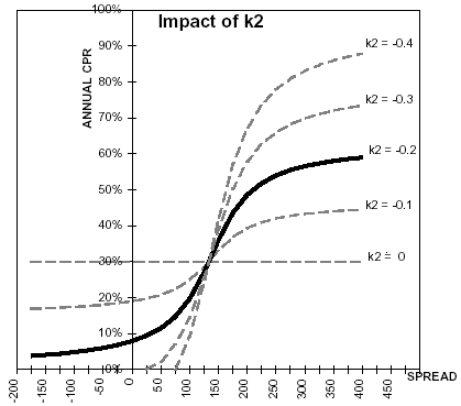
the picture is described in the document text

The following diagram shows the impact of K2 on the prepayment curve. K2 impacts the slope of the curve, defining the change in prepayments given a change in market rates. A larger value implies greater overall customer reaction to changes in market rates.

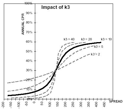
the picture is described in the document text

The following diagram shows the impact of K3 on the prepayment curve. K3 impacts the amount of torque in the prepayment curve. A larger K3 increases the amount of acceleration, implying that customers react more sharply when spreads reach the hurdle rate.

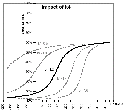
the picture is described in the document text

The following diagram shows the impact of K4 on the prepayment curve. K4 defines the hurdle spread: the spread at which prepayments start to accelerate. When the spread ratio = k4, prepayments = k1.

the picture is described in the document text

Related Topics

Prepayment Methodologies and Rules

Defining Prepayment Methodologies

Defining the Arctangent Method

Associating Node Level and Conditional Assumptions with Prepayment Rules

You can define prepayment methodologies at any level of the product hierarchy. Children of a hierarchical node automatically inherit the assumptions defined at the parent level. Methodologies directly defined for child nodes take precedence over those defined at the parent level. See: Defining Transfer Pricing Methodologies Using Node Level Assumptions.

You can also use the IF-THEN-ELSE logic of Conditional Assumptions to define prepayment methodologies based on particular characteristics of financial instruments. See: Associating Conditional Assumptions with Transfer Pricing Rules.

Related Topics

Setting Prepayment Rules

Setting and Executing the Transfer Pricing Process Rule

Setting and executing the Transfer Pricing Process rule is one of the mandatory steps in the Oracle Transfer Pricing process. The Transfer Pricing Process rule allows you to:

Submit transfer pricing, prepayment, and adjustment assumptions, respectively contained in the associated Transfer Pricing, Prepayment, and Adjustments rules, to the Transfer Pricing Cash Flow engine for processing.
Determine the data that you want to process in a particular run.
Define parameters used in transfer rate, option cost, and adjustment calculation, migration of transfer pricing results to the Management Ledger table, propagation, and auditing.
Choose the calculation mode for generating transfer pricing results, such as Remaining Term or Standard.
Select which calculations, such as, Transfer Rates or Option Costs, or both, should be performed.

Setting the Transfer Pricing Process rule is a two-step process. You need to first create a rule and then a version. The Transfer Pricing Process rule has a separate Run page. Once a Transfer Pricing Process rule has been created, a user may select Run to execute it. The Run page allows you to supply all the run time parameters to get the required results. See: Transfer Pricing Process Rules.

When a Transfer Pricing Process rule is executed, detail account records are processed and individual records are updated with the results of the transfer pricing process. These results are based on the process options selected.

The following table displays the Account table fields that may be updated as a result of transfer pricing processing when you select Account tables as the data source.

Account Table Fields Updated by Transfer Pricing Processing
Calculation Type	Calculation Mode	Account Table Field
Transfer Rates	Standard	Transfer_Rate and Matched_Spread
Transfer Rates	Remaining Term	Tran_Rate_Rem_Term
Option Costs	Standard	Historic_Static_Spread and Historic_OAS
Option Costs	Remaining Term	Cur_Static_Spread and Cur_OAS

Additionally, you may choose the Management Ledger table as the data source for transfer pricing certain products. If the Management Ledger table data source is selected, the following rows are created for each product:

Financial Element 170, Average Transfer Rate
Financial Element 450, Charge/Credit
Financial Element 172, Average Remaining Term Transfer Rate
Financial Element 452, Charge/Credit Remaining Term

Note: For a given combination of Company/Cost Center/Org and Line Item dimensions, only one row should exist for transfer rate (170 or 172) and charge/credits (450 or 452).
Financial Element 171, Historic Option Cost
Financial Element 451 Historic Option Cost Charge/Credit
Financial Element 173, Current Option Cost
Financial Element 453, Current Option Cost Charge/Credit

Important: Financial Element 140, Average Balance must exist in the Management Ledger table in order to successfully transfer price ledger balances.

Setting Transfer Pricing Rules

Transfer Pricing Rules

Setting Prepayment Rules

Prepayment Rules

Transfer Pricing Process Rule and Option Costs

Transfer Pricing Option Cost, Oracle Financial Services Reference Guide

Transfer Pricing Process Rule and Rate Index Rules

Rate Index Rules

Transfer Pricing Process Rule and Adjustments Rules

Adjustments Rules

Transfer Pricing Process Rule and Alternate Rate Output Mapping Rules

Alternate Rate Output Mapping Rules

Transfer Pricing Process Rule and Propagation Patterns

Propagation Patterns

Transfer Pricing Process Rule and Audit Options

Transfer Pricing Process Rule and Option Cost Parameters

In addition to transfer rates, the Transfer Pricing Process rule allows you to calculate the cost of options that are associated with the instruments. If you want to calculate option costs, you need to define the parameters used in options costing on the Transfer Pricing Process Version definition page. See: Transfer Pricing Process Rules.

The purpose of option cost calculations is to quantify the cost of optionality, in terms of a spread over the transfer rate, for a single instrument. The cash flows of an instrument with an optionality feature change under different interest rate environments and thus should be priced accordingly.

For example, many mortgages may be prepaid by the borrower at any time without penalty. In effect, the lender has granted the borrower an option to buy back the mortgage on par, even if interest rates have fallen in value. Thus, this option has a cost to the lender and should be priced accordingly.

In another case, an adjustable rate loan may be issued with rate caps (floors) which limit its maximum (minimum) periodic cash flows. These caps and floors constitute options.

Such flexibility given to the borrower raises the bank's cost of funding the loan and will affect the underlying profit. The calculated cost of these options may be used in conjunction with the transfer rate to analyze profitability.

Oracle Transfer Pricing uses the Monte Carlo technique to calculate the option cost. Oracle Transfer Pricing calculates and outputs two spreads and the option cost is calculated indirectly as a difference between these two spreads. These two spreads are:

Static spread
Option-adjusted spread (OAS)

The option cost is derived as follows:

Option cost = static spread -OAS

The static spread is equal to margin and the OAS to the risk-adjusted margin of an instrument. Therefore, the option cost quantifies the loss or gain due to risk. See: Transfer Pricing Option Cost, Oracle Financial Services Reference Guide.

Transfer Pricing Process Rule and Rate Index Rules

The Rate Index rule is one of the parameters that you need to define on the Transfer Pricing Process Version definition page to calculate option costs. See: Transfer Pricing Process Rules.

The purpose of the Rate Index Rule is to establish a relationship between a risk-free Interest Rate Code (IRCs) and other interest rate codes or Indexes. The Rate Index rule allows you to select the valuation curve that the system uses during stochastic processing. The Rate Index rule provides full support for multi-currency processing by allowing you to select one valuation curve per currency supported in your system. See: Rate Index Rules.

During the stochastic processing, the system generates future interest rates for the valuation curve you selected, which is then used to derive the future interest rates for any Index associated to that valuation curve based on the relationship you define. The rates thus forecasted for the IRCs or Indexes depend on the risk-free curve used for valuation of instruments associated with the derived IRCs or Indexes. As the risk-free rates change, the non risk-free interest rates change accordingly.

Transfer Pricing Process Rule and Adjustments Rules

Select an appropriate Adjustments rule on the Transfer Pricing Process Version definition page to calculate add-on rates and breakage charges. See: Transfer Pricing Process Rules.

The Adjustments rule lets you apply transfer pricing rate adjustments to an instrument record for purposes of determining specific charge and credit amounts. For example, you can apply adjustments for add-on rates (liquidity premiums, basis risk costs, pricing incentives to the line managers, other adjustments) and breakage charges.

Add-on rates and breakage charges related adjustments can be a fixed rate, a fixed amount, or formula based. These adjustments are calculated and output separately from the base funds transfer pricing rate, so that they can be easily identified and reported.

In addition, the Adjustments rule allows you to apply event-based transfer pricing adjustments through the use of conditional assumptions that are applied or varied only if a specific condition is satisfied. See: Adjustments Rules.

Transfer Pricing Process Rule and Alternate Rate Output Mapping Rules

Select an appropriate Alternate Rate Output Mapping rule on the Transfer Pricing Process Version definition page to output transfer pricing results to the seeded or user-defined alternate columns instead of default columns of the application. See: Transfer Pricing Process Rules.

The Alternate Rate Output Mapping rule lets you select the alternate columns to output transfer rate, option cost, and adjustment calculation results for each instrument record in an account table for a transfer pricing process run. This functionality allows you to output more than one transfer rate, option cost, or adjustment calculation result for each instrument record in the account table through multiple transfer pricing process runs.

For example, you may run Oracle Transfer Pricing once without selecting an Alternate Rate Output Mapping rule and thus use the original default output columns, such as such as TRANSFER_RATE and MATCHED_SPREAD, to output transfer pricing results. You may then run the application a second or third time using an Alternate Rate Output Mapping rule in different Transfer Pricing Process rules, which run against the same instrument records. The result would be two or three transfer rate, option cost, or adjustment calculation results populated into distinct columns for each instrument record in the specified account tables. See: Alternate Rate Output Mapping Rules.

Transfer Pricing Process Rule and Propagation Pattern

Transfer Pricing theory suggests that a Fixed Transfer Rate should apply to an instrument record throughout its entire life (for Fixed Rate Instruments) or Repricing Term (for Adjustable Rate Instruments).

Propagation Patterns allow you to move forward (propagate) the Transfer Rate and Matched Spread on any applicable instrument record from a prior period of history. Propagation methodologies are system specific and can be used across process rules. See: Propagation Patterns.

The Transfer Pricing Process Rule allows you to propagate Transfer Rates as well as Options Costs. Depending upon your requirements, you can choose to propagate either the transfer rate or the option cost or both on the Transfer Pricing Process Run page. See: Transfer Pricing Process Rules.

The main goal of using propagation is to increase performance. Since Propagation uses a bulk processing approach, it provides a significant performance improvement over processing instruments with a row-by-row approach. Although precise performance numbers may vary depending on the hardware and database configuration, processing a set of instrument records using propagation is significantly faster than doing it on the same set of records on a row-by-row basis.

Transfer Pricing Process Rule and Audit Options

The Transfer Pricing Process rules provides you with the three audit options: Detailed Cash Flow, Forward Rates, and 1 Month Rates. While Detailed Cash Flow audit option is applicable to both transfer rate and option cost processing, the Forward Rates and 1 Month Rates audit options are applicable only to option cost processing.

By selecting the Detail Cash Flow option in the Transfer Pricing Process Rule Run flow, you can audit daily cash flow results generated by the Oracle Transfer Pricing application. Selecting this option writes out all cash flow and repricing events that occur for processed records. The number of records written is determined by the environment on which the process is running. If you are running under multiprocessing, you may get fewer records, for example, OFSA_PROCESS_ID_STEP_RUN_OPT.NUM_OF_PROCESSES > 1.

The relevant financial elements for each instrument record and the cash flow results are stored in the FTP_PROCESS_CASH_FLOWS table, which is described in Oracle eBusiness Suite Electronic Technical Reference Manuals (eTRM).

After processing cash flows from Transfer Pricing, do the following to view the audit results:

Determine the value of Object ID. See: Executing a Transfer Pricing Process Rule.
View data by:
- Creating a Condition associated with the Object ID Number. See: About Conditions, Oracle Enterprise Performance Foundation User's Guide.
- Querying the FTP_PROCESS_CASH_FLOWS table with a Data Inspector rule to view the data. See: About the Data Inspector and Data Inspector Rules, Oracle Enterprise Performance Foundation User's Guide.

Note: Oracle Transfer Pricing has a seeded Oracle Discoverer workbook to help you query the cash flow audit results.

Data Inspector Results

The results of running the Data Inspector appear in a spreadsheet.

Financial Elements

The FINANCIAL_ELEMENT_ID column lists the financial elements written for each payment and repricing event processed by the cash flow engine. An initial set of data is also written, recording the balance and rate as of the last payment date.

The following table describes the financial elements that can be present in a base set of financial elements written during a cash flow audit process:

Financial Elements Written During Audit
Financial Element	Description
Initial Event
100	Ending par balance. Final balance on payment date, after the payment has occurred.
430	Interest cash flow.
210	Total principal runoff, including scheduled payments, prepayments, and balloon payments.
60	Beginning par balance. Starting balance and payment date, prior to payment.
120	Runoff Net Rate. Rate at the time of payment, weighted by ending balance. To view actual rate, divide financial element 120 by financial element 100.
490	(Stochastic Processes Only) Discount factor used during Monte Carlo process to determine present value of cash flow on the payment date.
Initial Event
250	Par balance at time of repricing.
280	Before Reprice Net Rate. Rate prior to repricing, weighted by reprice balance. To determine true rate, divide this financial element value by financial element 250.
290	After Reprice Net Rate. Newly assigned net rate after repricing occurs, weighted by reprice balance. To determine true rate, divide this financial element value by financial element 250.
Initial Event
100	Initial par balance at start of processing.
120	Initial net rate at start of processing.

Cash Flow Codes

The Cash Flow Code column lists a code for each row that describes the event modeled by the cash flow engine.

The following table describes the different cash flow codes:

Description of Cash Flow Codes
Cash Flow Code	Description
1	Initial recording of balances and rates.
2	Payment event only.
20	Reprice event only (not during tease period).
8	Reprice during tease period.
22	Reprice and payment event together (not during tease period).
10	Reprice and payment during tease period.

Data Verification

You can copy the results from the Process Cash Flows table and paste them into a spreadsheet to facilitate analysis against validated data. If the cash flows do not behave as expected, examine instrument table data or your assumptions. See: Cash Flow Calculations, Oracle Financial Services Reference Guide.

Transfer Pricing Process Rule and Calculation Modes

You can choose to transfer price your product portfolio either in the Standard or in Remaining Term calculation mode.

The Standard calculation mode allows you to calculate transfer rates for instrument records based on the Origination date or Last Repricing Date of the instruments. It can also be used to calculate Option Costs based on the Origination Date.

The Remaining Term calculation mode allows you to calculate transfer rates and option costs for instrument records based on the remaining term of the instrument from the calendar period end date of the data, rather than the Origination Date or Last Repricing Date of the instruments.

The Remaining Term calculation mode treats your portfolio as if you acquired it on the Calendar Period End Date of your data and thereby allows you to measure current rate risk spread. Once you know the current rate risk spread, you can segregate your total rate risk spread into that accruing from taking current rate risk and that accruing from taking embedded rate risk:

Embedded Rate Risk Spread = Total Rate Risk Spread - Current Rate Risk Spread

It is important to segregate total rate risk into embedded and current rate risks for the following reasons:

The current rate risk can be actively managed through an effective Asset/Liability Management process.
Embedded rate risk is a result of rate bets taken in the past. However, it is important to measure and monitor this risk. When you are aware of your embedded rate risk you will neither be lulled into a false sense of security or take drastic actions in response to profit or losses caused by the embedded rate risk.

See: Evaluating Interest Rate Risk, Oracle Financial Services Reference Guide.

Transfer Pricing Process Rule and Migration Options

The purpose of the Ledger Migration process is to generate dollar credits or charges for funds provided or used for a combination of dimensions. The information necessary to generate these credits or charges (through transfer rates and option cost processing) originates from the Customer Account Tables and the results are inserted into the Management Ledger table, and are available for use in calculation of profitability and risk measures.

Note: The Management Ledger table is also known as FEM_BALANCES and the Customer Account tables are also known as Instrument tables.

Oracle Transfer Pricing provides great flexibility in the ledger migration process and the generation of corresponding charges, credits, and option costs. Users can specify ledger migration for a combination of an extended list of dimensions, including up to 10 user defined dimensions. This feature enables the system with profitability reporting capabilities across organizational, product, channel, geography, and user defined dimensions.

Tip: Only the Management Table, FEM_BALANCES, processing key dimensions are available for inclusion during the migration process. This is because Oracle Transfer Pricing displays only the processing key dimensions on the user interface.

In addition, Oracle Transfer Pricing provides multi-currency support that allows you to generate charges or credits for funds based on entered and functional currency. See: The Ledger Migration Process, Oracle Financial Services Reference Guide.

You can choose to migrate either the transfer rate or the option costs, or both, on the Transfer Pricing Process rule run page. See: Transfer Pricing Process Rules.

Defining Payment Patterns

A prerequisite for transfer pricing your product portfolio is capturing instrument behavior, such as payment and repricing patterns. This is because transfer rate and option cost processing require cash flow generation, which is possible only if you have accurately captured the payment and repricing profiles of the products in your portfolio.

The payment and repricing patterns for most instruments can be accommodated in the Account tables. However, certain instruments may have payment and repricing patterns that are too complex to be accommodated in the standard fields of Account tables. Oracle Transfer Pricing allows you to define custom payments and repricing patterns for such instruments. See: User Defined Payment Patterns and User Defined Repricing Patterns.

In a user defined payment pattern, you can assign a unique amortization code to a set of payment events, which may include some of the following customized features:

Changes in payment frequency
Seasonal payment dates
Nonstandard or variable payment amounts

Once you create a payment pattern, you can use it by entering the payment pattern code as the amortization type code for the instrument.

Defining Repricing Patterns

Payment Pattern Structure

Oracle Transfer Pricing allows you to build three types of payment patterns:

These payment patterns differ in terms of how they address payment schedules, which determine whether the payment events constituting the pattern are determined by calendar dates or periods. Absolute patterns are defined with sets of payment characteristics scheduled on specific calendar dates. Relative patterns are defined with sets of payment characteristics scheduled for certain periods of time.

You can also define a payment pattern with both absolute and relative payment events. This type of pattern is called a split pattern.

In addition, for each payment pattern, you need to specify a payment type, either conventional, level principal, or non-amortizing. Your choice of the pattern type and the payment types will determine the fields that are used for calculation.

Note: Oracle Transfer Pricing's Payment Pattern interface supports simultaneous multiple-user access.

Related Topics

Defining Payment Patterns

User Defined Payment Patterns

Payment Events

You must define one or more payment events to complete a payment pattern. A payment event is a set of payment characteristics, which define the time line and amount of a specific payment in the payment pattern.

Though the characteristics of the payment phase change based on whether you are defining an absolute, relative, or split pattern, there are two characteristics that are required for all amortizing patterns:

Payment method
Value

Payment Method

The payment methods determine the payment amount for the payment event. There are six different methods.

The following table describes the different payment methods.

Payment Methods
Method	Description
% of Original Balance	This method calculates the payment as a percentage of the original balance; the percentage being defined by the input percent. This method is useful for apportioning the starting balance on a level principal instrument over several payments. This method is only available for payment patterns defined with a level principal payment type.
% of Current Balance	This method calculates the payment as a percentage of the current balance prior to payment; the percentage being defined by the input percent. This method is only available for payment patterns defined with a level principal payment type.
% of Original Payment	This method calculates the payment as a percentage of the original payment column from the detail instrument data. This percentage is defined by the input percent.
% of Current Payment	This method calculates the payment as a percentage of the previous payment; the percentage being defined by the input percent. This payment is calculated on the payment date based on the characteristics of the instrument at the time of the payment, including the current rate, current balance, and current payment frequency.
Absolute Payment	This is an input payment amount. This amount represents both principal and interest for a conventional payment type, and represents only principal for a level principal payment type. For both types of patterns, absolute value payment amounts are entered as gross of participations.
Interest Only	This is a calculated payment amount. An interest-only payment is calculated during processing as balance times rate times accrual factor.

Value

The value reflects the percentage or payment amount based on the method chosen for the payment event. Value is disabled for phases using the Interest Only payment method.

Payment amounts for conventional pattern phases must reflect both principal and interest payments. Payment amounts for level principal pattern phases only reflect the principal portion of the payment. For level principal pattern phases, the total cash flow on a payment date is the principal amount stored as the payment plus the calculated interest.

Note: The payment method and value columns are not displayed for payment patterns defined with a non-amortizing payment type. All payments are assumed to be interest only for this type of payment pattern.

Related Topics

Defining Payment Patterns

User Defined Payment Patterns

Absolute Payment Patterns

Absolute payment patterns are commonly used for instruments that are on a seasonal schedule, such as agricultural or construction loans that require special payment handling based on months or seasons.

Take the example of a loan that follows a seasonal payment pattern, in which the payment patterns for January, February and March are scheduled for interest-only payments. As revenues for the customer increase, the payment amount also increases. Therefore, the payments for April and May are 80% of the original payment, and June through September is 100% of the original payment. The payment decreases as the production season slows. The payment for October is decreased to 80% of the original payment, and the payments for November and December are decreased again to 50% of the original payment.

See: Defining Absolute Payment Patterns.

Note: You can define absolute payment patterns only up to a year. This is because all entries are automatically ordered by date and are scheduled in a single year rotation.

Related Topics

Defining Payment Patterns

User Defined Payment Patterns

Relative Payment Patterns

Relative payment patterns are commonly used for modeling instruments with irregular payment frequencies or for instruments where the payment type changes over time.

Take the case of a four-year loan for example. The payment for the first 12 months could only be interest. The first 35 payments are scheduled for 50% of the currently scheduled payment, and the last payment is a balloon payment for the balance of the loan.

See: Defining Relative Payment Patterns.

Related Topics

Defining Payment Patterns

User Defined Payment Patterns

Split Payment Patterns

A split pattern contains multiple sets of payment patterns under a single amortization code. You use a split pattern for financial instruments that make principal payments along two concurrent amortization schedules. Each separate amortization schedule is termed a time line and assigned a percentage of the balance. A Split Pattern can constitute both absolute and/or relative payment patterns within itself. See: Defining a Split Payment Pattern.

Related Topics

Defining Payment Patterns

User Defined Payment Patterns

Defining Repricing Patterns

User defined repricing patterns provide a mechanism to capture the repricing structure of instruments whose rates change according to complex schedules which cannot be captured in the standard fields of account tables. See: User Defined Repricing Patterns and User Defined Payment Patterns.

The user defined repricing pattern allows you to define multiple changes to various elements affecting repricing including:

Rates
Margins
Frequency

A repricing pattern has two major components:

Note: Oracle Transfer Pricing Repricing Pattern interface supports simultaneous multiple-user access.

Defining Payment Patterns

User Defined Repricing Pattern

The user defined repricing pattern provides you with the ability to define a series of repricing patterns and events that describe the interest rate adjustment characteristics over the life of a cash flow instrument. One repricing pattern can be assigned to many cash flow instruments.

There are two types of repricing patterns that you can define:

See: Creating a Repricing Pattern.

Related Topics

Defining Repricing Patterns

User Defined Repricing Patterns

User Defined Repricing Event

The events of a repricing pattern define changes to the interest rates of an instrument during its life. Every pattern begins with an initial event, which describes the behavior for the initial period.

Note: This initial event is required for the setup of all repricing patterns but is not used in Oracle Transfer Pricing. This feature is used only by Risk Manager, another Oracle Financial Services application, when assigning a rate at origination of new business and transaction strategy records.

The second event describes the change in behavior after the initial period is over. A third event describes the next change in behavior and so on. In relative repricing patterns, you can also define the number of times an event will be repeated before the next event is triggered.

At least one event must be defined for a repricing pattern. All events are listed in the Repricing Events table. The repricing pattern type, absolute or relative, determines the data required to be populated in the events table.

Caution: You have the option to change the repricing pattern type at any time during the create process. However, changing the repricing pattern type causes the system to automatically refresh the Repricing Events table, and the loss of all the data that you previously entered.

Event Detail

You define each event with a repricing type of either flat rate or indexed rate. The repricing types determine the event detail characteristic that are available.

Flat Rate

Selecting the flat rate repricing type allows you to set the rate of the instrument to a fixed value. For example, 6%.

The following table describes the event detail characteristics that are available when the flat rate repricing type is selected.

Event Detail Characteristics: Flat Rate
Characteristic	Description
Net Rate	The new net rate value
Gross Rate	The new gross rate value
Transfer Rate	The new transfer rate

Flat rate always overrides the caps and floors defined on the instrument record.

Indexed Rate

Selecting the indexed rate repricing type allows you to set the rate of the instrument to an adjustable value, defined as the index rate plus a margin.

The following table describes the event detail characteristics that are available when the indexed rate repricing type is selected:

Event Detail Characteristics: Indexed Rate
Characteristic	Description
Interest Rate Code	Reference interest rate used as the index rate to set gross and net rates. This list of values is pulled from the current Historical Rates database.
Transfer Interest Rate Code	Interest rate used to calculate transfer rate. The field is a list of value type.
Net Margin	Added to index rate to get net rate.
Gross Margin	Added to index rate to get gross rate.
Transfer Margin	Added to index rate to get transfer rate.
Rate Cap Life	The upper limit for gross rate set by a particular event.
Rate Floor Life	The lower limit for gross rate set by a particular event.
Rate Set Lag	Period by which the date of the interest rate used for calculation precedes the event date; set with a value and a multiplier.
Yield Curve Term	Term used in interest rate code lookups; if left blank, defaults to the term until the next repricing; set with a value and multiplier.

Related Topics

Defining Repricing Patterns

User Defined Repricing Patterns

Absolute Repricing Pattern

The absolute repricing pattern is used for instruments that are date dependent. Each specific date is a separate event.

You may have up to one year of defined events that repeat for the life of the instrument. For example, you could define one event for each day of the year; the maximum number of events that you can define is 365. However, you can only define one event for any given date. See: Defining Absolute Repricing Pattern.

Related Topics

Defining Repricing Patterns

User Defined Repricing Patterns

Relative Repricing Pattern

The relative repricing pattern is a series of repricing events that are driven by user defined time lines. It is used for instruments where the repricing is determined by elapsed time since origination. You specify the duration of each repricing period (frequency) and the number of times that event should occur (repeat) before calculating the next event in the pattern.

For example, an event can be defined with a frequency of 1, a multiplier of Months, and a repeater of 3. This translates into an event that reprices every month for a duration of 3 consecutive months.

You may have a graduated rate mortgage that requires three rate changes over the life of the instrument. You will have three events following the initial event. If you wish the instrument to retain the behavior defined for the last event, the repeater should be set to 999. This prevents wrapping, or the repetition of all the defined events until the life of the instrument runs out. See: Defining Relative Repricing Pattern.

Related Topics

Defining Repricing Patterns

User Defined Repricing Patterns

Performing Cash Flow Edits

It is extremely important that the data in Account tables is clean, accurate, and complete before it is used to generate cash flows and for further processing. Oracle Transfer Pricing provides Cash Flow Edit rules to edit (clean and prepare) Account table data. You can create multiple Cash Flow Edit rules depending on the data to be cleansed. In addition, you can view actual results of Cash Flow Edits by accessing the result data written into the FTP_CF_CORRECTIONS table.

You can also select the preview option so that you can preview the changes that will be made to the Account table data as a result of cash flow edits before those changes are applied in the account tables.

It is highly recommended that you create and run Cash Flow Edit rules before processing data to generate any type of cash flow-related results. See: Cash Flow Edits Rules.

Creating Interest Rate Codes

Oracle Transfer Pricing uses historical interest rate information to transfer price your balance sheet. The final transfer rate assigned to the instruments in your account tables is based on the historical rates information stored in the system. Consequently, you must decide on the type and amount of historical rate information you require to satisfy your transfer pricing requirements at the outset of an Oracle Transfer Pricing implementation.

However, the quality and availability of interest rate information varies throughout the world. In many markets, gathering comprehensive rate information is a challenge because of insufficient security types, inconsistent quoting conventions, and lack of liquidity. This necessitates careful management of the interest rate data. In Oracle Transfer pricing, this is done using reference interest rates, called interest rate codes.

Creating interest rate codes is one of the mandatory steps in the Oracle Transfer Pricing process. Oracle Transfer pricing provides a separate rule, called Interest Rate Codes (IRC), to define and manage historical interest rates for transfer pricing purposes.

Oracle Transfer Pricing facilitates the process of inputting and viewing interest rates by giving you data storage capabilities appropriate to your market. This is possible as the application supports multiple rate formats and allows you to store the following rate attributes:

Rate format (zero-coupon or yield-to-maturity)
Accrual basis
Compound basis

In addition to historical interest rate information, Oracle Transfer Pricing allows you to manage the term structure modeling parameters, such as volatility and mean reversion speed. See: Interest Rate Codes.

Interest Rate Codes and Rate Lookups

A rate lookup is performed to derive a transfer rate for the appropriate date/term combination.

Date Used: Oracle Transfer Pricing accesses the yield curve based on the appropriate lookup date. If no match is found, it uses the first date before the date of your lookup.

Term Used: Oracle Transfer Pricing selects the term on the yield curve on an exact number of days basis, calculated by subtracting the cash flow date from the transfer pricing date, which may be the calendar period end date, the last reprice date, or the origination date depending on the method and the instrument characteristics.

If the yield curve term is expressed in months or years, the term must be converted to a days basis, as follows:

If Multiplier = M (month), Term in Days = Term in Months * 30.42

If Multiplier = Y (year), Term in Days = Term in Years * 365

The rate is then derived from the yield curve by performing linear interpolation to the two points between which the lookup term falls.

Rate Lookup at Endpoints

If the term < shortest point on the yield curve, then the rate = the shortest point.

If the term > longest point on the yield curve, then the rate = the longest point.

If the date for the lookup > dates available then the lookup is on the last date for the yield curve.

If the date for the lookup < dates available then the lookup is on the first date for the yield curve.

Rate Lookup: An Example

The following table displays transfer rates for different date/term combinations:

Date	1 Day	1 Month	3 Months	1 Year
01/01/2004	2.00	3.00	4.00	5.00
01/15/2004	2.10	3.10	4.10	5.10
01/31/2004	2.20	3.20	4.20	5.20
02/15/2004	2.30	3.30	4.30	5.30

The following table displays Date/Term Combinations for Lookup:

Date	Lookup Term	Yield Curve Date Used	Term Before	Term After	Rate	Comments
01/07/2004	60 days	01/01/2004	1 Month	3 Months	3.50	Rate is approximately half way between 3 Months (91.26 Days) and 1 Month (30.42 Days).
11/30/2003	182 days	01/01/2004	3 Month	1 Year	4.33	3 Months Rate + (182 Days - 91.26 Days) * (1 Year Rate - 3 Months Rate) / (365 Days - 91.26 Days) (such as 1/3 of the Way between 3 Months and 1 Year).
03/15/2004	2 Year	02/15/2004	1 Year	None	5.30	Uses last point on Yield Curve.

Accessing Transfer Pricing Detail Cash Flow Results for Audit Purposes

Detailed cash flow results for individual account records can be written to an audit table for validation purposes. If you select the Detailed Cash Flows audit option on the Transfer Pricing Process rule run page, the detailed cash flow results are written to the FTP_PROCESS_CASH_FLOWS table, which is described in Oracle eBusiness Suite Electronic Technical Reference Manuals (eTRM).

Accessing Transfer Pricing Interest Rate Audit Results

Forward Rates and 1 Month Rates audit results can be written to an audit table to facilitate validation of option cost results.

On the Transfer Pricing Process rule run page, selecting the Forward Rates option allows you to audit the static spread calculations, and the 1 Month Rates option allows you to audit the option-adjusted spread calculations by writing out the different paths of one-month rates. Since 360 one-month rates are written out for each rate path, the process might be lengthy.

The Forward Rates and 1 Month Rates audit results are written to the FTP_INTEREST_RATES_AUDIT table, which is described in the Oracle eBusiness Suite Electronic Technical Reference Manuals (eTRM).

Analyzing Results

You should always analyze results obtained from the Transfer Pricing engine. For example, you should review the historical rates information (Interest Rate Codes) to ensure that the new cost of funds reflect the current interest rate reality.

In addition, a detailed transfer rate/matched spread query should be generated at the product level to ensure that every account has been assigned a transfer rate and that the matched spread for each account is as expected.

The following table lists some steps to find out whether an account has not been transfer priced correctly:

Steps to Analyze Transfer Pricing Results
Query	Results
Stratification by transfer rate	Look for any transfer rate <= a selected value (such as 3.00) or >= another value (such as 12.00)
Stratification by matched spread	Look for large (positive or negative) matched spreads. (for example, >= 4.00 or <= -2.00)
Stratification of fixed rate instruments by origination date and term with weighted average transfer rate and matched spreads as columns	Look for general pattern to reflect the Transfer Pricing Yield Curves for each origination date
Stratification of adjustable rate instruments by last repricing date and term with weighted average transfer rate and matched spreads as columns	Look for general pattern to reflect the Transfer Pricing Yield Curves for each last repricing date

In case a result (transfer rate) generated by the system is suspect, then you can view all of the cash flows for any specified instrument record, by selecting the Detailed Cash Flow option in the Transfer Pricing Process rule. This option should be selected together with a condition, which identifies the instruments to be included in the Audit process.

After ensuring that each account has been assigned an accurate transfer rate, you should review the funding center impact and compare it to the results from prior periods.

Reviewing Processing Errors

There is always the possibility that errors might occur during the execution of a Transfer Pricing Process rule. A log of such errors is generated during processing and can be accessed from within the concurrent manager. Within this log, the application identifies the specific transaction for which an error was generated and provides the internally generated identifier of the Transfer Pricing Process rule that generated it.

As part of the rectification process, it is advisable to determine what caused the error and what should be done to correct it for the next run.

Reprocessing Erroneous Accounts

While reviewing your results, you might discover accounts with invalid results that need to be reprocessed. The Transfer Pricing Process rule allows you to rerun a subset of information.

If you need to reprocess a portion of your instrument data, make sure that you reprocess all the Line Item dimensions members for a rule. Otherwise, you may damage your overall results.

If any of the records being reprocessed are used as the basis for unpriced accounts, those unpriced accounts also should be reprocessed.

Reconciling the Data

Reconciliation is the process of comparing the information carried in the Account tables to the general ledger.

The goal of the Transfer Pricing Process rule is to transfer price your entire balance sheet, as represented on the general ledger. Many ledger accounts have corresponding data in the Account tables. In such instances, the balances from the instrument data must be compared with the corresponding ledger balances.

The reconciliation process involves defining a level at which some piece of information in the Account tables is to be compared to the General Ledger data carried in the Management Ledger (also known as FEM_BALANCES, and formerly known as Ledger Stat) table. That level can be one dimension (to reconcile for each general ledger account number, for example, Natural Account ID) or multiple dimensions (to reconcile for each general ledger account number within each business unit, for example, Natural Account and Company Cost Center Org ID).

The most common type of reconciliation is to compare the current balance of Account table data to the general ledger ending balance. The data carried in the database is a snapshot of the portfolio as of a given date. Consequently, comparing the current balances from the Account table to the general ledger ending balance measures the degree to which the extracted data is in balance with, or reconciles to, the general ledger.

Variances between the Account table and the Management Ledger table should be corrected. If the magnitude of the variances is high, plug entries should be created to force the reconciliation to zero.