Analyzing Data
This chapter covers the following topics:
Overview of Analyzing Data
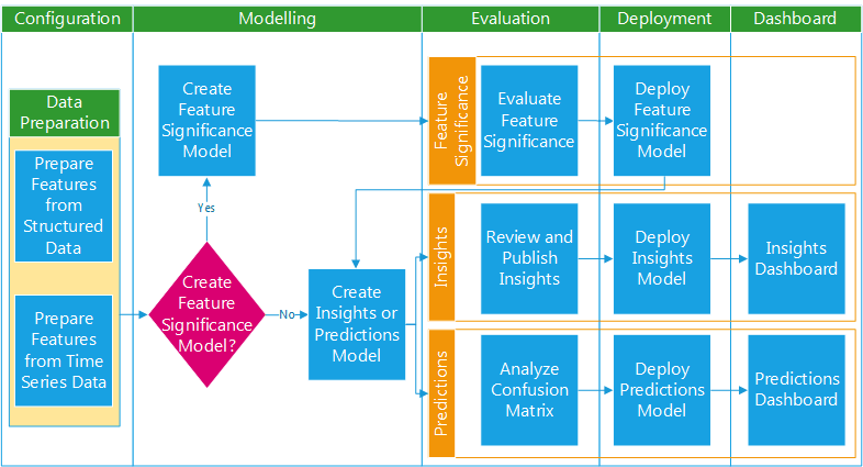
The process of successfully creating a dataset extracts features from structured data and time series data. You can then analyze the data by applying data mining techniques to form deeper insights into improving target measures for products. The data mining process typically starts with building a statistical model that uses an algorithm on a set of data which contains a set of input features and a specific target variable. The model building process consists of the following steps:
-
Creating a model.
-
Evaluating a model.
-
Deploying a model.
Model Building Flow
Analyzing Insights or Predictions Models Using Custom Key Performance Indicators
When creating an insights or predictions model, you have the option to select target measures associated with custom key performance indicators (KPIs). This enables you to analyze custom KPIs such as Cycle Time, Machine Efficiency, Machine Downtime and so on.
These target measures defined as custom KPIs can also be used in models to analyze the effect of flex attributes associated with business entities, such as the lot expiry date associated with a lot or the voltage associated with an operation.
Related Topics
Defining Key Performance Indicators
Overview of Importing Business Entity Data, Oracle Adaptive Intelligent Apps for Manufacturing Data Ingestion User's Guide
Creating a Model
You can build different models to achieve different purposes, such as understanding the significant features or analyzing the relationship between a specific target measure and the features selected. When you create a model you select the type of model, the target measure, features, algorithm, and deployment options. The model then creates a data set by extracting data from different work orders for the selected features and the output target measure, running the algorithm on the data extracted.
You can choose from the following three analysis types:
-
Feature significance model - analyzes data and extracts the most influential features that potentially impact a given target measure.
-
Insights model - identify patterns and correlations between the influencing factors and the output target measure. You can either select features from the ranked features generated from the Feature Significance model or select features that you are interested in for the analysis.
-
Predictions model - identifies conditions under which predictions are made for a target variable by considering various input variables/predictors. You can either select features from the ranked features generated out of the Feature Significance model or select features that you are interested in for the analysis.
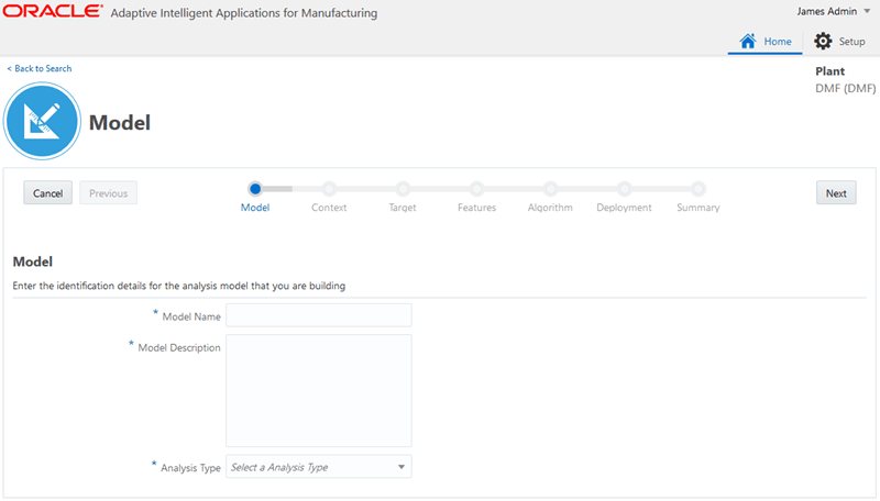
To create a model
-
Navigate to the Model page.
From the Home page, click Predictions or Insights, and then Modeling.
The existing models appear in the Model page.
-
Click Create.
-
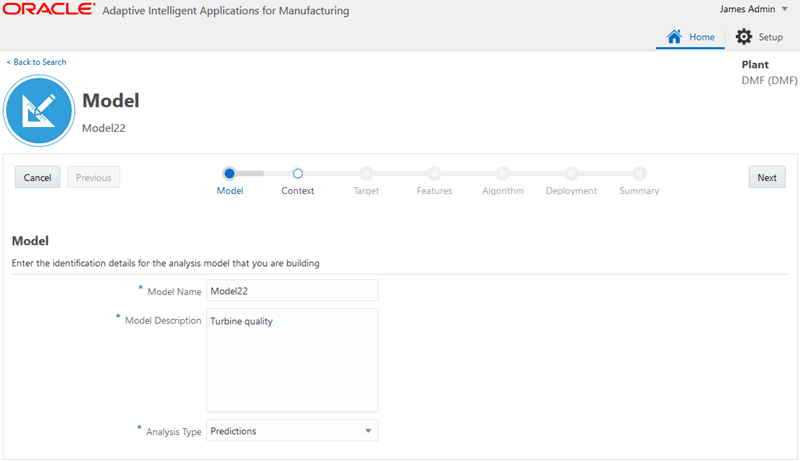
Enter the following model details:
-
Model Name - use only alphanumeric characters and the special characters #, $, and _.
-
Model Description
-
Analysis Type - select the type of model to create.
-
Feature Significance
-
Insights
-
Predictions
-
-
-
Click Cancel to cancel the process. To continue, click Next.
-
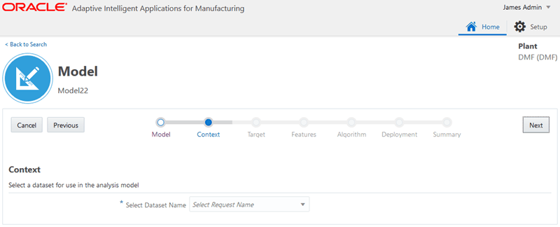
Select Dataset Name from the list in the Context section.
Choose the request name of a dataset that you previously created.
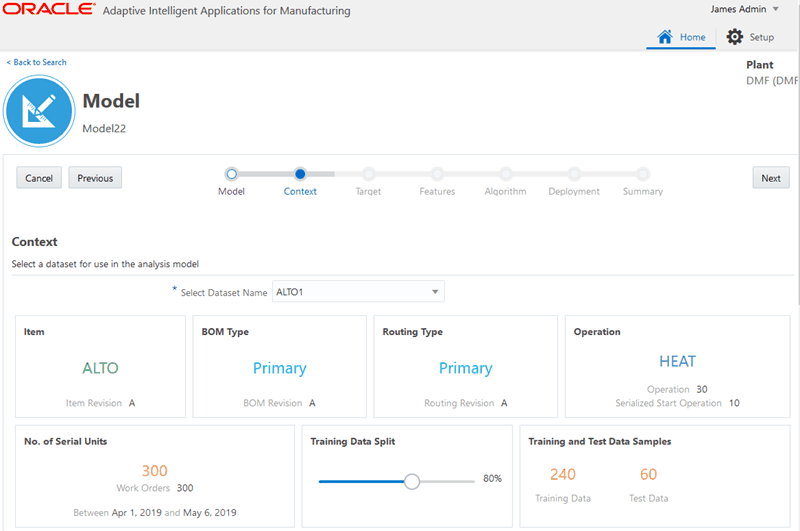
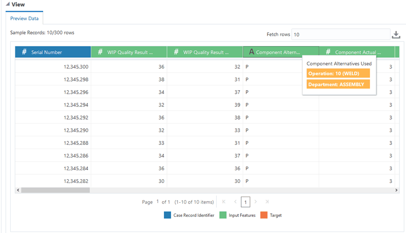
After you select a dataset, you can scroll to view information in the Preview Data tab.
Tip: Preview the data for multiple datasets. Use the Select Dataset Name field to select and preview various datasets while on this page.
For Predictions models only
-
Specify the Training Data Split.
Use the slider to split the training and test data from the sample. The Predictions module uses the training data to train and build the model and uses the test data to evaluate the model performance. The default slider setting is 80% training data and 20% test data. However, you can use the slider to select a training sample between 50-100% of the input data.
The Predictions module uses stratified sampling to proportionately split data into training and test samples. This homogeneous splitting of the data ensures equal representation of the data in both training and test samples.
-
-
Click Cancel to cancel the process. Click Previous to go back to the Model step. To continue, click Next.
-
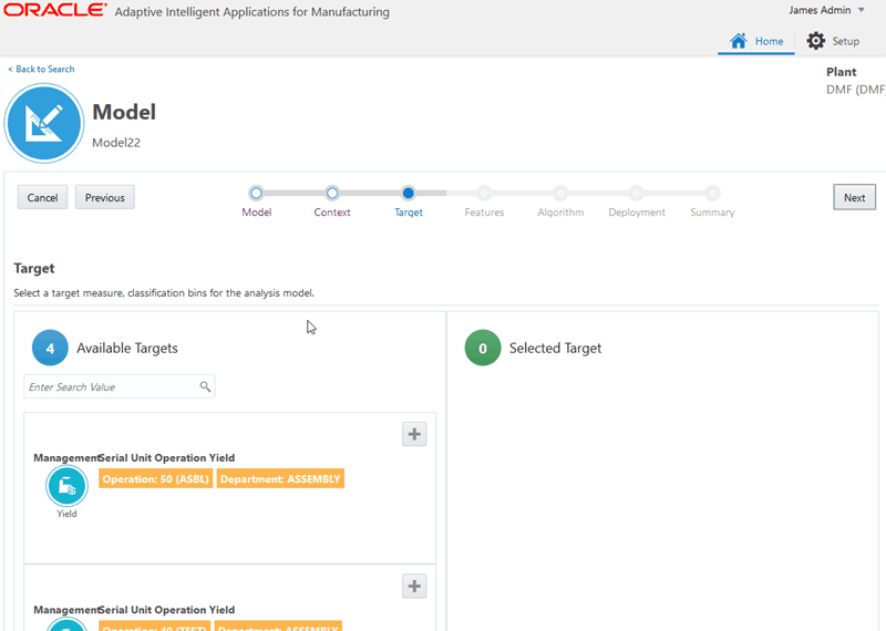
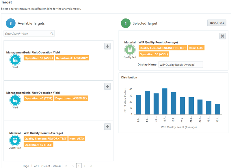
Select a target measure for the model from the list of available targets.
-
Optionally, change the selected target Display Name.
-
Define bin limits if none exist. Edit the bin limits, if needed. Click either Define Bins or the Edit icon.
-
Serialized analysis models with a yield target display the following seeded bins:
-
Feature Significance models: Pass and Fail bins.
-
Predictions models: Pass and Fail bins.
-
Insights models: Accepted With First Pass, Pass With Rework, Rejected, and Scrapped bins.
-
-
For a Predictions model, you have the option to turn on alerts on the Bins page for certain classification ranges. If actual results fall within these classification ranges, predictions/alerts appear on the Predictive Analysis page. See: Using Predictions Analysis.
-
Define a minimum of two bins for all other types of targets.
-
-
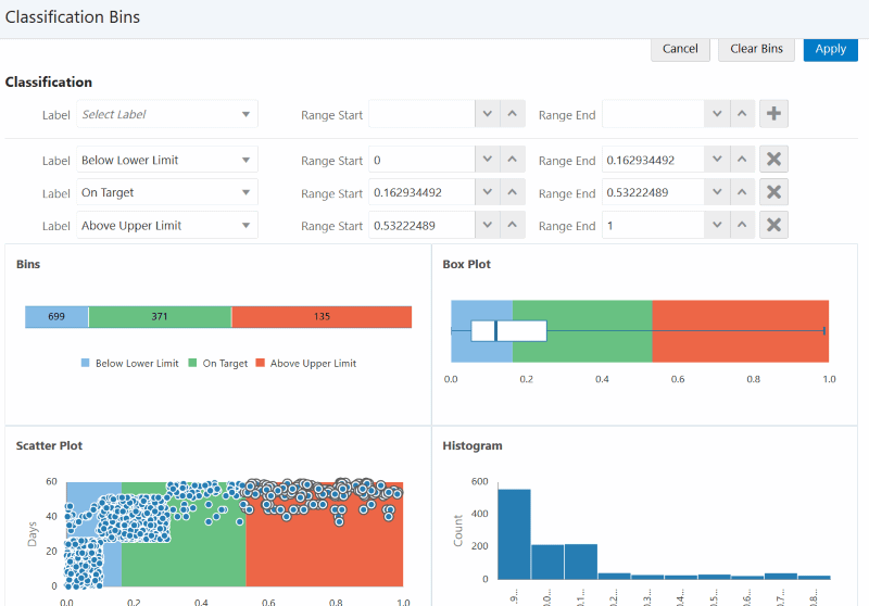
Add a new classification label and range, delete an existing classification label, or update the range of an existing label. Optionally, click Clear Bins to clear the bin range selection and remove the bin coloring from the charts.
The following charts appear in the Update Bins page:
-
Bins: Displays the total number of case records.
-
Box Plot: Displays the distribution and quartiles.
-
Scatter Plot: Displays the distribution of target attribute data points and plots these points based on the case record day scale along the Y axis.
Note: If there are more than 10,000 data points, stratified sampling is applied before displaying the scatter plot.
-
Histogram: Displays the frequency distribution of data points. Up to 10 frequency ranges are used to plot the histogram.
Notice that the Bins, Box Plot, Scatter Plot, and Histogram charts change along with any classification changes made. Use the plus icon to add at least two classification ranges. The model predicts outcomes based on the ranges defined. For example, the model predicts a classification range, such as Low, Medium, or High, not a specific number, such as 84.6.
-
Add classification ranges using the pre-defined labels provided.
-
You can save the classification bins when:
-
No gaps exist between the ranges. An unclassified range (gap) appears as white space in the Bins, Box Plot, and Scatter Plot charts.
-
Each data point falls within a classification range.
-
Each classification range contains at least one data point.
-
Classification ranges do not overlap.
Tip: To view the number of data points in each new or updated classification range, click the Show Count link in the Bins chart region.
-
-
A data point is classified under a classification range if the Range Start <= data point < Range End, except for the last classification range where range end is also considered. For example, if you define the Low range as 0 to 20 , the Medium range as 20 to 80 and the High range as 80 to 100, then a result of 20 is classified in the Medium range and a result of 100 is classified in the High range.
Tip: Define a new classification range by dragging a selection area over unclassified data points in the Scatter Plot or use the Histogram as a visual aid while entering ranges.
-
-
Click Apply.
The system returns to the Model page, Target step.
-
Click Cancel to cancel the process. Click Previous to go back to the Context step. To continue, click Next.
-
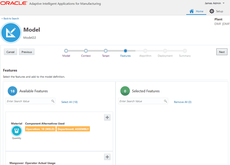
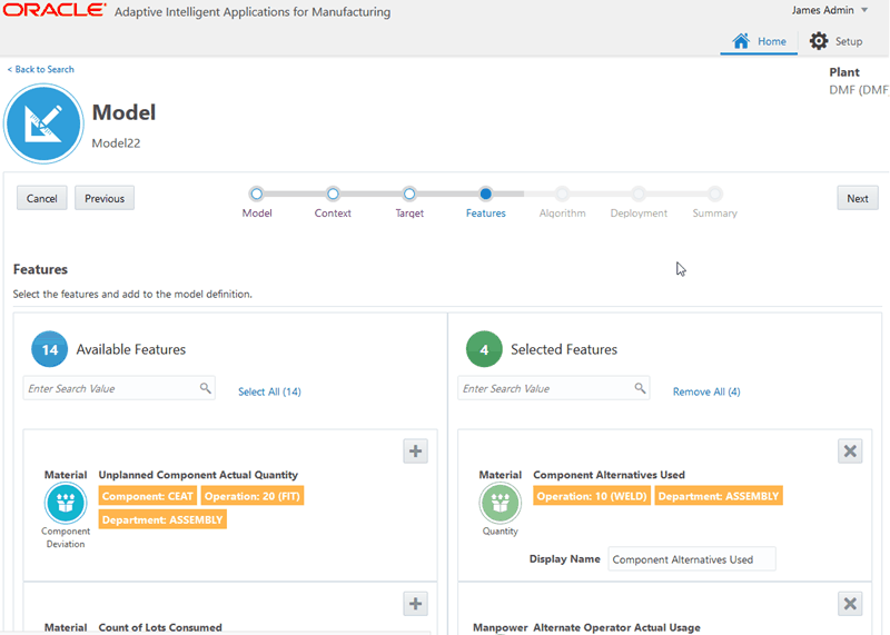
Search for and select the features to use as predictors in the model.
Refer to Model Predictors for Process Manufacturing or Model Predictors for Discrete Manufacturing for a description of each feature.
-
Use the Available Features field to search for features.
-
Each feature may appear as an available feature multiple times, depending on the occurrence of the feature in the operations. For example, an operation duration feature appears for multiple operations.
-
Click the Feature Significance link for a feature to view the feature's statistics.
-
If you previously deployed a feature significance model that used the same context (dataset) as the Insights or Predictions model you are creating, then the Ranked Features box is checked so you can easily select the ranked features as predictors. Deselect Ranked Features to view all other available features extracted in the dataset.
-
-
Click Cancel to cancel the process. Click Previous to go back to the Target step. To continue, click Next.
-
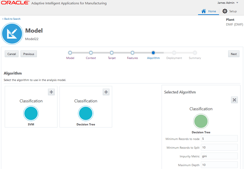
Select an algorithm for the model.
Note: The algorithm choices vary depending on the model analysis type selected and certain algorithms have parameters that you can change. For more information about a particular algorithm, see:
-
Click Cancel to cancel the process. Click Previous to go back to the Features step. To continue, click Next.
-
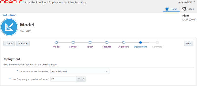
Select whether or not to deploy the model.
Selecting Auto Deploy deploys the model once it is built. You can only auto-deploy Feature Significance and Insights models. These two types of models only run once after deployment. If a Feature Significance or Insights model has been previously created using the same context and deployed, then Auto Deploy defaults to off.
For a process manufacturing Predictions model, select from the following deployment options:
-
When to start the Prediction?
-
Step status becomes In Process - start when the step begins.
-
Step status becomes Pending - start when the batch begins.
Warning: Do not select this deployment option when using the case record data ingestion method. This ingestion method only brings in historical work orders and in progress work orders, not pending work orders, or operations that are pending.
-
x minutes after Step status becomes In Process - start x minutes after the step begins.
-
-
How frequently to Predict? - select the frequency of prediction in minutes.
For a discrete manufacturing Predictions model, select from the following deployment options:
-
When to start the Prediction?
-
Job is released - start when the job is released.
-
Assembly is in process at Operation - start when the operation begins.
-
Assembly is at Operation - start before the operation begins.
Warning: Do not select this deployment option when using the case record data ingestion method. This ingestion method only brings in historical work orders and in progress work orders, not pending work orders, or operations that are pending.
-
-
How frequently to Predict? - select the frequency of prediction in minutes.
-
-
Click Cancel to cancel the process. Click Previous to go back to the Algorithm step. To continue, click Next.
-
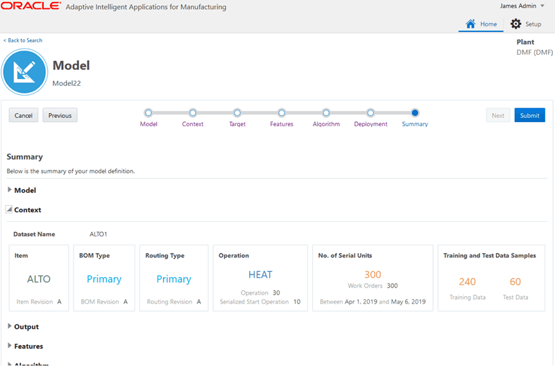
Review the model definition. You can choose to redefine the model using the previous pages.
Click Cancel to cancel the process. Click Previous to go back to the Deployment step. To continue, click Submit.
-
When you submit the model, the system returns you to the Modeling page and the status of your request appears as IN PROGRESS.
Confirm that the status of the model changes to COMPLETED. Should the model status be in ERROR, navigate to the Background Process page to view the run details. See: Running Background Processes.
Alternatively, you can copy an existing model using the Copy Model icon. When copying a model, the original model's options are chosen by default, but you can change the model name, the training data split, the selected target and bins, the selected features, the algorithm, and deployment options from the original model's definition.
-
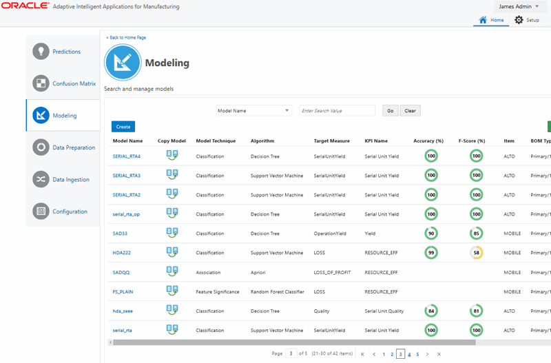
Navigate to the Model page.
From the Home page, click Predictions or Insights, and then Modeling.
The existing models appear in the Model page.
-
Click the Copy Model icon next to the model name that you want to copy.
-
Optionally, change the Model Name and Model Description.
The model name defaults to the original model name, appended with "_1". For example, a copy of "model name" is named "model name_1".
-
On the Context page, for Prediction models only, optionally adjust the previously set training data split. Click Next.
-
The target from the original model displays on the Targets page. Optionally, add new bin ranges to the existing target or add a new target from the list of available targets.
-
Click Bins.
Optionally, modify the bins for existing targets and define bins for new targets. You can also change the display names of selected targets and set turn classification bin alerts on or off.
-
Click Next.
-
On the Features page, optionally remove existing features, add new features, and change the feature display names.
-
Click Next.
-
On the Algorithm page, optionally change the selected algorithm's parameter values or select another algorithm.
-
Click Next.
-
On the Deployment page, optionally change the original deployment options.
-
Click Next.
-
On the Summary page, review your selections for each model definition area. Click Previous to change your selections or click Submit.
Evaluating a Model
After building various models that use different parameters, input features, and algorithms or algorithm parameters to predict a specific target measure, you can evaluate each model to determine which model best fits historical data. Data scientists evaluate each functional type of model differently.
-
Feature Significance - Evaluate how much each feature influences target measure results. Use the most significant features to create your Insights and Predictions models.
-
Insights - Discover patterns in the historical work order data and publish the insights that influence the business outcome with a high level of factors influence.
-
Predictions - Evaluate and review the performance of a predictions model using the confusion matrix. This matrix displays total predictions generated for the model and the percentage of true and false predictions by comparing predictions with actual results.
To evaluate a feature significance model
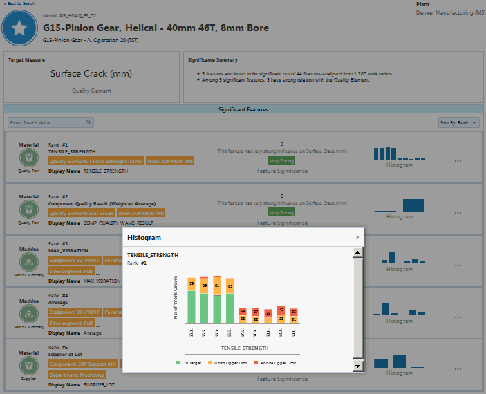
Use the Feature Significance page to determine which features in your feature significance model have a significant relationship with the model's target measure.
-
Navigate to the Feature Significance page.
From the Home page, click Insights, then Evaluation, and then Feature Significance.
-
Click View in the Significant Features column for a model.
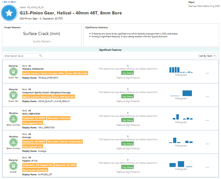
The resulting page displays feature significance details for the selected model. This page displays:
-
the target measure.
-
a Significance Summary, which explains the number of significant features versus the number of features analyzed in comparison to a set of historical results data. If the model uses the Chi Square algorithm, there is also an explanation of how many significant features have a strong relation to the target measure.
-
a Significant Features region, which provides a ranked and analyzed list of significant features.
Tip: Search for significant features using the Search field in the top left corner of the Significant Features region. The search criteria include:
-
Categories
-
Subcategories
-
Features
-
Entities
-
Relationships/Reasons
Sort the significant features using the Sort By field in the top right corner of the Significant Features region. You can sort features by:
-
Rank
-
Category
-
Name
View Significant Features page
-
-
In the third column of the Significant Features region, view the following information about each feature:
-
If the model uses the Chi Square algorithm, a statement explains the strength of the feature's influence on the target measure. For example, in the screen shot shown above, the statement says "This feature has very strong influence on Surface Crack (mm)".
-
If the model uses the Random Forest Classifier algorithm, a number, ranging from 0 to 1, represents the importance of the feature's influence on the target measure. This number is displayed using a meter gauge format.
-
Click the bar chart for a feature to view a histogram showing how the feature's historical data falls within the model's classification ranges.
Histogram
-
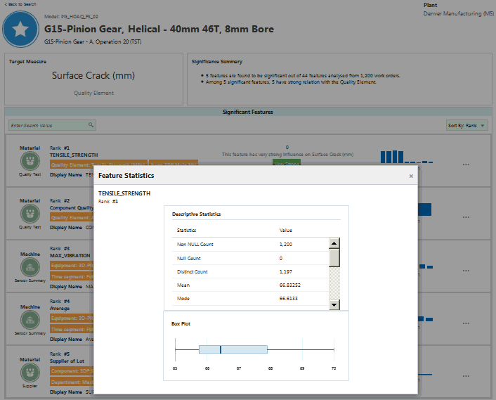
Click the ellipsis points ( . . . ) on the right side of each significant feature listed to view the Feature Statistics page. This page includes the descriptive statistics of the feature and a box plot showing the data distribution for the selected feature.
-
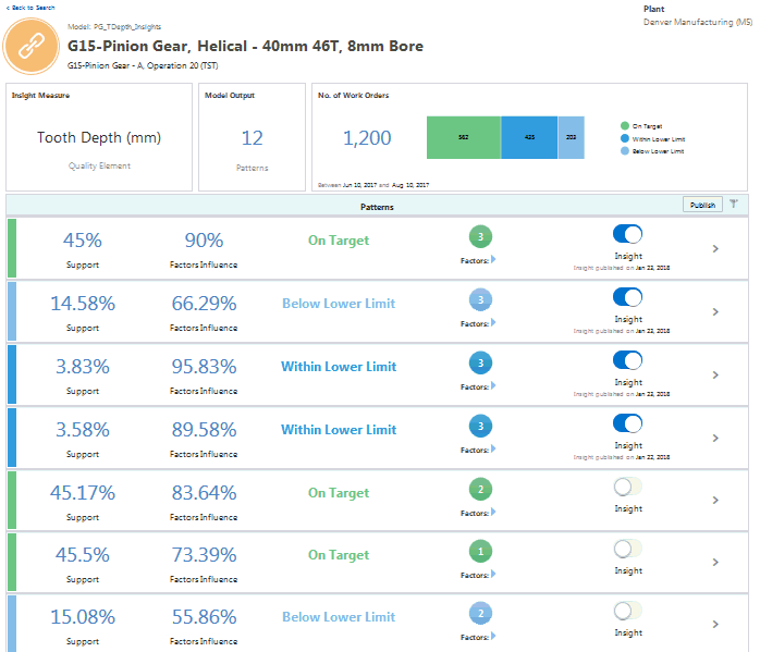
Navigate to the Patterns & Correlations page.
From the Home page, click Insights, then Evaluation, and then Patterns & Correlations.
-
Click View for a particular model name.
-
Review the results for the model:
-
Insight Measure - the measure for which the model discovers influencing factors.
-
Model Output - the number of patterns (insights) found by the model. The model discovers various patterns/correlations between influencing factors and the target measure selected for the model.
-
Number of Work Orders - total number of historical work orders analyzed by the model. The chart provides a distribution of test results for the predefined classification ranges. For serialized manufacturing, the number of serial units and the distribution of test results of serial units by predefined classification range displays.
View Significant Features page
-
-
Review the results for each insight.
You can choose to publish up to ten insights for a given model. The top ten insights are selected for publishing by default. You can choose to modify the selections. Before publishing, review the support and factors influence percentage parameters for each pattern to determine which of them most influence the target measure. You must also apply your understanding of the business when determining which patterns to publish as insights to the end users in the Insights module pages. For each pattern, review:
-
Support - the percentage of historical work orders supporting the pattern out of the total number of work orders analyzed.
-
Factors Influence - the percentage of historical work orders that match the pattern out of all the historical work orders that match only the input factors.
-
Factors - the number of factors which influenced the target measure to have a classification as discovered in the insight model.
-
-
Click the right arrow underneath the number of features to display the list of features.
-
Click the right arrow on the right side of the insight row to view the following charts:
-
Insight Measure Classification - displays the number of historical work orders where:
-
an insight pattern exists. The total number of work orders where the insight pattern exists (having both the input feature and the insight measure or the target measure matching as per the insight).
-
the input features match. The total number of work orders where only the input features match as per the insight but the target measure or the insight measure values are different from that of the insight..
-
a pattern does not exist. The total number of work orders where both the input feature and the target measure values do not match with the insight.
-
-
Correlation - correlation or distribution chart displaying the correlation (scatter plot) or distribution (bubble chart) between each influencing factor of the insight versus the target measure.
-
Insight Timeline - displays the target measure value information for all work orders matching the insight along a timeline. The target measure values are legends with the classification labels.
-
To evaluate a predictions model
-
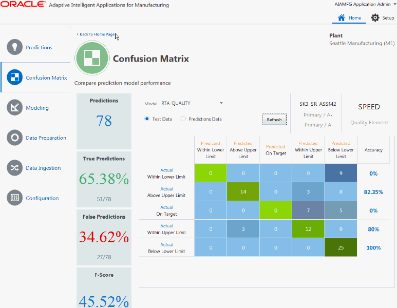
Navigate to the Confusion Matrix page.
From the Home page, click Predictions and then Confusion Matrix.
-
Select the model to evaluate.
-
Select Test Data, then click Refresh.
The test data is a portion of the data set on which the model is tested. When the model is built, the data set is split into training data and test data. The model is created using the training data, but evaluated against the test data.
In the example Confusion Matrix table shown below, the model generated:
-
Predictions: 78 predictions of the quality element SPEED from the test data.
-
True Predictions: 65.38% true predictions (percentage of predictions that matched actual results).
-
False Predictions: 34.62% false predictions (percentage of predictions that did not match actual results).
-
F-Score: 45.5%.
The F-Score measures a model's accuracy, with a range between 0 - 100%. The higher the F-Score, the more accurate the model. The F-Score is computed as a harmonic mean between precision and recall. Use it as metric to evaluate model performance in cases of uneven class distribution or imbalanced data sets.
The matrix displays the predictions and compares them with actual results for each classification. The model shown below generated 12 Within Upper Limit SPEED predictions, but the SPEED of the assembly was actually within the upper limit 3 more times, for a total of 15 times. The accuracy of predictions are displayed by each classification.
Note: You can also evaluate a predictions model using the most recent data once the actual work order results are available. To do this, run the program "Update Actuals for Prediction Model Targets" before evaluating the predictions model against the predictions data. For more information about this program, see Background Processes.
Example Confusion Matrix Table
-
-
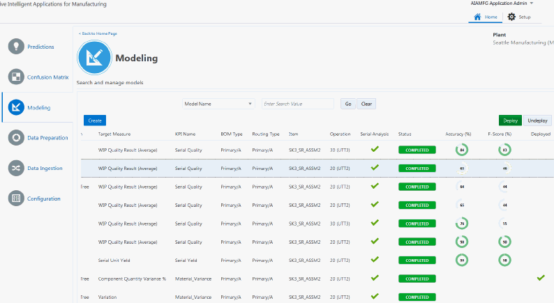
Navigate to the Modeling page.
From the Home page, click Predictions and then Modeling.
-
Search for the predictions models that you want to compare.
-
Evaluate the models based on their Accuracy (%) and F-Score (%).
Deploying a Model
To deploy a feature significance model
Although you can create many feature significance models that use the same dataset and target measure, you can only deploy one of them at a time.
-
Navigate to the Feature Significance page.
From the Home page, click Insights, then Evaluation, and then Feature Significance.
-
If multiple models for a certain context (which includes the dataset) and a target measure exist, decide which model to deploy.
-
Select the row for the model that you want to deploy.
-
Click Deploy.
A green check mark appears in the Deployed column upon successful deployment.
Warning: If you previously deployed another model with the same context and target measure, you must undeploy it before deploying another model. Select the row for the previously deployed model, then click Undeploy.
To deploy an insights model
Insights models have an auto-deploy option which is enabled for the initial insights model of a given dataset and target measure combination. Upon deployment of an insights model, the insights are published and appear on the Insights page. Each deployed model must contain at least one insight. Oracle recommends deploying an insights model only after evaluation. See: Evaluating a Model.
-
Navigate to the Patterns & Correlations page.
From the Home page, click Insights, then Evaluation, and then Patterns & Correlations.
-
Select the row for the model that you want to deploy.
-
Click Deploy.
A green check mark appears in the Deployed column upon successful deployment.
Note: You can deploy multiple Insights models with the same context and target measure. If you want to undeploy a model, select the row for the previously deployed model, then click Undeploy.
To deploy a predictions model
-
Navigate to the Modeling page.
From the Home page, click Predictions, then Modeling.
-
Select a Predictions model row.
Tip: Select a Predictions model based on the model's accuracy and F-score.
-
Click Deploy.
A green check mark appears in the Deployed column upon successful deployment.
Additional Information: If you previously deployed a model with the same context and target measure, you must undeploy it before deploying another model. Select the row for the previously deployed model, then click Undeploy.
When you deploy a Predictions model, the Run Predictions Model background process starts and runs on the frequency specified in the Deployment option. Note that if a predictions model is currently running for any in-progress work orders, you cannot undeploy the model. In such cases, use the Background Process page to cancel the Run Predictions Model program, and then undeploy the model. See Running Background Processes for information about how to cancel the predictions process or modify the predictions schedule.