| Oracle® Retail Demand Forecasting User Guide for the RPAS Fusion Client Release 16.0 E91109-03 |
|

 Previous |
 Next |
| Oracle® Retail Demand Forecasting User Guide for the RPAS Fusion Client Release 16.0 E91109-03 |
|
Previous |
Next |
This chapter discusses the forecasting methods used in Oracle Retail Demand Forecasting in detail.
RDF uses a variety of predictive techniques to generate forecasts of demand. The technical methods used are driven by the goal to provide the most accurate forecasts possible in an automatic and efficient manner. These methods have been analyzed, optimized, and refined over years of research on retail-specific data.The primary techniques RDF uses include:
Exponential smoothing models fit basic features of the demand pattern such as level, trend, and seasonality, and project these into the future. These models provide computational benefits and have been chosen for their ability to handle different types of time series, including short and/or noisy series that are characteristic of retail sales. They are smoothing models because they use weighted averages on historic data. They are exponential smoothing models because the weighting uses decays at an exponential rate. That is, more recent data is weighted more heavily than the past.
Regression analysis is another standard technique used in prediction. Regression uses a least-squares estimator to fit a model of predictor variables to another set of target variables. Seasonal Regression is an Oracle Retail specific extension of this procedure for use in seasonal models with between one and two years of history. Causal Forecasting uses stepwise regression to determine which causal variables are significant.
Bayesian analysis considers a priori information as a starting point in development of a prediction. Bayesian forecasting, as developed by Oracle Retail, uses a sales plan as the starting point that is adjusted based on observed data. This method fills a gap in standard time series forecasting when new, short lifecycle or products with significant lifecycles are being forecast.
Predictions from these various models gives the estimated mean outcome. By using standard statistical distributional assumptions, RDF develops measures of uncertainty associated with forecast point estimates from these models. While this is of key concern for various optimization solutions of the forecast, the technical details are beyond the scope of this document. For further details on prediction interval calculations, refer to Char&Yatfield, International Journal of Forecasting, March 1992.
Providing multiple forecasting methods is only valuable if the appropriate model can be selected in an accurate and efficient manner. In order to make this feasible in a retail environment, Oracle Retail has developed a number of different meta-methods that can automatically select the best method among a number of competing models. Automatic Exponential Smoothing (AutoES) is an example of one such method that clients can select. The final selection between the competing models is made according to a performance criterion that involves a trade-off between the model's fit over the historic data and its complexity. A description of the competing models used within AutoES is described in "Exponential Smoothing (ES) Forecasting Methods". In academia, this discipline is known as Information Theory and is used in the combination and selection of various competing models.
Sometimes it is difficult to capture seasonality, trend, or causal effects on the final-level (item/store) due to scarcity of the data. Also, time series are often too noisy at that level. To overcome these issues, RDF utilizes source-level forecasting. In source-level forecasting, data is aggregated first to a higher level across the product or location hierarchy (or both). Then the forecast is generated and proportionally spread down to the final-level. We have experimentally proven that source-level forecasting technique often improves the accuracy on the final-level.
In some instances, especially in retail, pure time series techniques are inadequate for forecasting demand. Instead of using only historic demand patterns to forecast future demand, additional causal or promotional factors are used to better explain past performance. With the help of a promotional calendar, an indication of when promotions is run in the future, these promotional forecasting techniques can better predict demand in the future.
This section describes those techniques within RDF that generate forecasts directly from only a single time series. Generally the time series provided is past sales history for a given item/store that is used to predict what future demand might be. In actual practice these algorithms have been and can be used to forecast a myriad of different data streams at any product/location level (shipment data at item/warehouse, financial data at dept./chain, and so on).
The following topics present fundamentals of the RDF statistical forecasting processes. Included is a discussion of the importance of confidence intervals and confidence limits, the time series methods used to generate forecasts, and how the best forecasting method is selected from a list of candidate models.
A wide variety of statistical forecasting techniques are available, ranging from very simple to very sophisticated. All of these methods attempt to best capture the statistical probability distribution previously discussed, and they do this by fitting quantitative models to statistical patterns from historical data. Put simply, the better the history of the variable being forecast, the stronger these statistical patterns are. Increased forecast accuracy depends on the strength of these patterns in relation to background irregularities.
RDF is able to use several time series methods to produce forecasts. Time series methods extrapolate features from the past (in this case, past sales data) to the future. The time series methods that the system offers include:
Average (Simple Moving Average)
Exponential Smoothing (ES) Forecasting Methods - Automatic Exponential Smoothing (AutoES)
The purpose of statistical forecasting is to make the process of predicting future events both objective and quantitative. Statistical forecasting utilizes information from the past (such as sales data) to predict what will happen in the future. Forecast accuracy depends on the degree to which a mathematical model can detect and extract statistical patterns from historic data. The most common statistical methodologies used are univariate. This means that they are based solely on the history of one variable, such as sales. Each forecast observation reflects a future value of the sole input variable. Statistical forecasting processes are relatively easy to implement, and the better the historical data, the better the resulting forecasts.
Businesses benefit greatly from the use of systematic statistical forecasting techniques that aim to accurately predict product demand, enabling these businesses to maintain sufficient product inventory levels. When inventory levels are optimized, lost sales due to product stock-outs are greatly reduced, as are the costs incurred by overstocking.
A simple moving average forecast involves taking the average of the past n time periods and using that average as the forecast for all future time periods (where n is the length of fitting period). Simple moving average forecasts are frequently used in the system because they:
Make few assumptions about the historical time series.
Can be generated with little historical data.
Are very fast to generate.
Typically, moving average forecasts are generated at the final forecast level (for example, item/store) and their results used to spread more sophisticated higher-level forecasts (for example, those generated with exponential smoothing).
A Simple Moving Average model assumes that historical data is too short or noisy to consider seasonal effects or local trend and is based on the level of the series. Since this model does not use a smoothing parameter to place added weight on more recent historic values, a Simple Moving Average model is not actually in the exponential smoothing family. However, it is an adequate model to use when low-level (final forecast) ratios are needed for RDF's spreading of high-level (aggregate) forecasts. That is, when aggregate forecasts can be calculated for long and less noisy aggregate time series, Simple Moving Average models provide an adequate (and computationally quick) forecast to determine the ratios needed for RDF spreading. User input in overriding the automatic training horizon further enhances the simple robustness of this model for base-level data.
Within AutoES, the model that minimizes the Bayesian Information Criterion (BIC) is selected as the final model. The BIC criterion attempts to balance model complexity with goodness-of-fit over the historical data period (between history start date and forecast start date). The BIC criterion rewards a model for goodness-of-fit and penalizes a model for its complexity. The complexity penalty is necessary to avoid over fitting.
There are various equivalent versions of the Bayesian Information Criterion, but RDF minimizes the following:
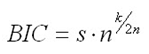
where n is the number of periods in the available data history, k is the number of parameters to be estimated in the model (a measure of model complexity), and s is the root mean squared error computed with one-step-ahead forecast errors resulting from the fitted model (a measure of goodness-of-fit). Note that since each member of the model candidate list is actually a family of models, an optimization routine to select optimal smoothing parameters is required to minimize s for each model form (that is, to select the best model).
Within RDF, a few modifications to the standard selection criteria have been made. These include reducing the number of parameters the Winter's model is penalized by discounting seasonal indices that have little impact on the forecast (multiplicative indices close to one (1), additive indices close to zero (0)). These changes tend to favor the seasonal models to a slightly higher degree that improves the forecasts on retail data, especially for longer forecast horizons.
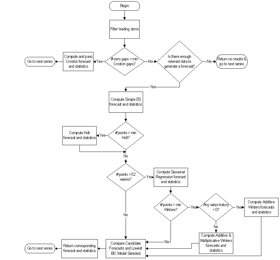
The following procedure outlines the processing routine steps that the system runs through to evaluate each time series set to forecast using the AutoES method. Refer to Figure 3-1, "AutoES Flowchart".
Filter all leading zeros in the input data that is within the training window.
Does the time series contain the minimum data points to qualify to forecast using the Croston's method? If yes, generate the forecast and statistics using the Croston's method and move on to the next time series. If no, move on to Step 3.
Does the time series contain enough relevant data to generate a forecast? If yes, generate a forecast and statistics using the SimpleES method and move on to Step 4. If no, do not forecast and go to the next time series.
Does the time series contain the minimum data points to qualify to forecast using the Holt method? If yes, generate a forecast and statistics using the Holt method and move on to Step 5. If no, move on to Step 9.
Does the time series contain more than 52 weeks of input data? If yes, generate a forecast and statistics using the Seasonal Regression method and move on to Step 6. If no, move on to Step 9.
Does the time series contain the minimum data points to qualify to forecast using Winters methods? If yes, move on to Step 7. If no, move on to Step 9.
Does the time series contain any data point with sales equal qualify to forecast using Additive Winters method? If yes, generate the forecast and statistics using the Additive Winters method and move on to Step 9. If no, move on to Step 8.
Does the time series qualify to forecast using the Multiplicative Winters method? If yes, generate the forecast and statistics using both the Additive Winters and Multiplicative Winters methods and move on to Step 9.
Compare all candidate forecasts using BIC Criterion.
Return the corresponding forecast and statistics for the system-selected forecast method and move on to the next time series.
This section describes how the automatic forecast level selection (AutoSource) could help improve the accuracy of your forecasts.
In the system, one of the key elements to producing accurate forecasts is using the system's ability to aggregate and spread sales data and forecasts across the product and location hierarchies. Low selling or relatively new products can use aggregated data from similar products/locations at a higher level in the hierarchy, generate forecasts using this data, and then spread these higher level forecasts back down to provide more accurate forecasts. The difficulty comes in deciding which products/locations will benefit from this technique and from what level in the hierarchy these source-level forecasts should be spread.
The Automatic Forecast Level Selection feature of the system automates the selection of best aggregation level (forecast source-level) for each product/location combination. While providing invaluable information regarding the best aggregate level for source forecasts, the Automatic Forecast Level Selection process may be very CPU intensive. To solve this problem, the task of selecting best aggregation levels for product/location combinations is decomposed and processed piecemeal during times when the computer would normally be idle.
Identifying the best aggregation levels for sets of products and locations can be divided into a number of sub-problems:
Forecasting
Determining the best source-level forecast
Status and scheduling
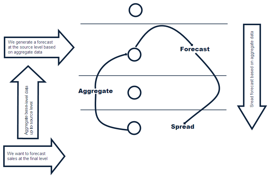
The automatic source generation level selection subsystem selects the best source generation level for each product/location in a given final forecast level. In order to determine the best level, a final forecast is generated for each product/location using each candidate source generation level. As illustrated in Figure 3-2, a final forecast is generated by:
Aggregating up from the base level to the source-level
Generating a source-level forecast
Spreading the source-level forecast down to the final-level
For example, assume base-level sales data is at the item/store level, the final forecast level is at the item/store level, and the candidate source generation level is at the style/store level. In this case, base-level sales data is aggregated from the item/store level up to the style/store level. A style/store forecast is generated, and the forecast data is spread back down to the item/store level. This forecast represents the final forecast.
The selection of the best level is based on a train-test approach. In this process, historical data is used to generate a forecast for a test period for which actual sales data already exists. The forecast, generated over the train period, can be compared to the actual sales figures in the test period to calculate the Percent Absolute Error (PAE) between the two.
A final-level forecast is generated for each product/location combination using each potential source generation level. Each time a source-level forecast is generated, a PAE is calculated for that level. If that PAE is better than the current best PAE (corresponding to the current best source generation level), the source generation level that generated that better PAE becomes the new best level.
Identifying the best aggregation level for a given set of products and locations may take a significant amount of time (that is, an amount of time that is greater than the duration of the computer's shortest idle period). This task, however, can be partitioned meaning that the problem of selecting the best aggregation levels can be decomposed into smaller sub-problems to be solved piecemeal during times when the computer would normally be idle.
For each product/location combination at the final forecast level, the problem consists of:
Generating forecasts at each unique aggregation level
Using the train-test approach to evaluate the percent absolute error statistics for each
One or more of these subtasks is performed during each period that the computer is idle. The best aggregation status keeps track of which sub-problems have been performed and which sub-problems remain. In this way, when the best aggregation procedure is run, the procedure knows what the next sub-problem is.
Best aggregation level procedures are run during idle computer periods. The scheduling of the Automatic Forecast Level Selection process (AutoSource) must be integrated with the schedules of other machine processes. In general, you should select a schedule so that source generation-level selection does not conflict with other activities. The following is an example of a typical schedule for the Automatic Forecast Level Selection process: Monday through Thursday, the selection process starts at midnight and runs for eight hours. On Friday and Saturday, the process is allowed to run for 20 hours. Sunday is reserved for generating forecasts.
You have the option of accepting the system-generated source-level selection or manually selecting a different source-level to be used. The value for the source forecast level can be manipulated in the Final Level view of the Forecast Maintenance workbook. For each product/location combination, the best source forecast level identified by RDF appears in the Optimal source-level measure on this view. You can enable the use of this level by placing a check mark in the Pick Optimal Level measure for that product/location. The absence of a check mark in this measure causes the system to default to the Default Source level or the Source Level Override value if this has been set by you.
The primary process by which RDF automatically fits an exponential smoothing model to a time series is called Automatic Exponential Smoothing (AutoES). When AutoES forecasting is chosen in RDF, a collection of candidate models is initially considered. The models in the candidate list include:
These models include level information, level and trend information, and level, trend and seasonality information, respectively. The optimal smoothing parameters for each model form are determined automatically (that is, greater smoothing is applied to noisier data). The final selection between the resulting models is made according to a performance criterion that involves a trade-off between the model's fit over the historic data and its complexity.
The amount of available historic information can affect the complexity of the model that can be fit. For example, fitting a seasonal model would not be appropriate without a complete year of historic data. In fact, one prefers to see each season occur multiple times. For a particular series, even if the amount of available history allows one to fit a complex model (that is, one with seasonal components), the resulting model is not necessarily superior to a simpler model. If a simpler model (for example, a model with only a level component or level and trend components) fits as well as a seasonal model, the AutoES forecasting process finds the simpler model to be preferable. In such a case, the simpler model captures the basic features supported by the data without over fitting and therefore generally projects better forecasts.
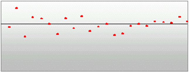
Simple Exponential Smoothing does not consider seasonality or trend features in the demand data (if they exist). It is the simplest model of the exponential smoothing family, yet still adequate for many types of RDF demand data. Forecasts for short horizons can be estimated with Simple Exponential Smoothing when less than a year of historic demand data is available and acts-like associations are not assigned in RDF.
Figure 3-3 is an example of a forecast in which data seems to be un-trended and un-seasonal; note the flat appearance of the forecast.
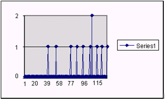
Croston's method is used when the input series contains a large number of zero data points (that is, intermittent demand data). The method involves splitting the original time series into two new series:
Magnitude series
Frequency series
The magnitude series contains all the non-zero data points, while the frequency series consists of the time intervals between consecutive non-zero data points. A Simple Exponential Smoothing model is then applied to each of these newly created series to forecast a magnitude level as well as a frequency level. The ratio of the magnitude estimate over the frequency estimate is the forecast level reported for the original series.
Figure 3-4 shows a sales history of data where the demand for a given period is often zero.
This method is a combination of the SimpleES and Croston's (IntermittentES) methods. The SimpleES model is applied to the time series unless a large number of transitions from non-zero sales to zero data points are present. In this case, the Croston's model is applied.
Holt exponential smoothing treats data as linearly trended but non-seasonal. The Holt model provides forecast point estimates by combining an estimated trend (for the forecast horizon - h) and the smoothed level at the end of the series. RDF uses a damped Holt model that decays the trend component so that it disappears over the first few weeks. This improves forecasts created using Holt over longer forecast horizons.
When this forecasting method is selected, the forecasts are seen as trending either up or down, as shown in Figure 3-5.
Overall, a forecast point estimate is evaluated as:
a function of level, trend, seasonality, and trend dampening factor.
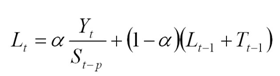
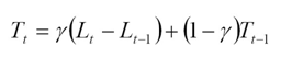
The Level at the end of the series (time t) is:
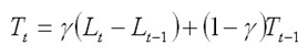
The Trend at the end of the series (time t) is:
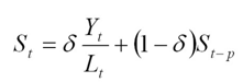
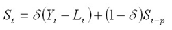
The Seasonal Index for the time series (applied to the forecast horizon) is:
Oracle Winters, calculates initial seasonal indices from a baseline Holt forecast. Seasonal indices, level, and trend are then updated in separate stages, using Winter's model as a basis for the updates.
Oracle Winters is the current seasonal forecasting approach, which uses a combination of Winters approach and decomposition. Decomposition allows level and trend to be optimized independently while maintaining a seasonal curve.
From sufficient data, RDF extracts seasonal indexes that are assumed to have multiplicative effects on the de-seasonalized series.
|
Note: The component describing the de-seasonalized values, which is multiplied by the seasonal index: is the Holt model previously described. is the Holt model previously described.
In this case, three parameters are used to control smoothing of the components of level, trend, and seasonality. |
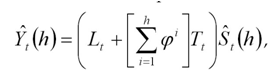
When the Multiplicative Seasonal forecasting method is selected, the forecasts tend to look squiggly, as shown in Figure 3-6.
Overall, a forecast point estimate is evaluated as:
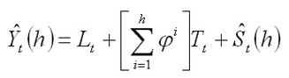
a function of level, trend, seasonality and trend dampening factor.
The Level at the end of the series (time t) is:
and the Trend at the end of the series (time t) is:
and the Seasonal Index for the time series (applied to the forecast horizon) is:
Oracle Winters is a Winters-based decomposition approach to update the level, trend, and seasonal indexes.
Refer to Multiplicative Winters Exponential Smoothing in this document for a description of each of the forecasting approaches.
A combination of several seasonal methods. This method is generally used for known seasonal items or forecasting for long horizons. This method lets the Multiplicative Seasonal and Additive Seasonal models compete and picks the one with the better fit. If less than two years of data is available, a Seasonal Regression model is used. If there is too little data to create a seasonal forecast (in general, less than 52 weeks), the system selects from the Simple ES, Trend ES, and Intermittent ES methods.
A common benchmark in seasonal forecasting methods is sales last year. A sales last year forecast is based entirely on sales from the same time period of last year. Forecasting using only sales last year involves simple calculations and often outperforms other more sophisticated seasonal forecasting models. This method performs best when dealing with highly seasonal sales data with a relatively short sales history.
The seasonal models used in earlier releases of RDF (Additive and Multiplicative Winters) were designed to determine seasonality. However, they were not designed to work with sales histories of shorter than two years. Because sales histories of longer than two years are often difficult to obtain, many retail environments need a seasonal forecast that can accommodate sales data histories of between one and two years. In addition, the Additive and Multiplicative Winters models search for short-term trends and have difficulties with trends occurring inside the seasonal indices themselves.
The current RDF Seasonal Regression forecasting model is designed to address these needs.
The Seasonal Regression Model uses simple linear regression with last year's data as the predictor variable and this year's sales as the target variable. The system determines the multiplicative and additive weights that best fit the data on hand. When optimizing the Seasonal Regression Model, the sales last year forecast is inherently considered, and it will automatically be used if it is the model that best fits the data. If there have been significant shifts in the level of sales from one year to the next, the model learns that shift and appropriately weigh last year's data (keeping the same shape from last year, but adjusting its scale).
As with other seasonal models, you can forecast demand for products with insufficient sales histories using this method if:
You paste in fake history as needed, providing a seasonal profile for the previous year.
You also forecast for a source-level (with the same seasonality profile as the forecast item and with more than one year of history) using seasonal regression and spread these forecast results down to the member products.
The Seasonal Regression Model is included in the AutoES family of forecasting models and is thus a candidate model that is selected if it best fits the data.
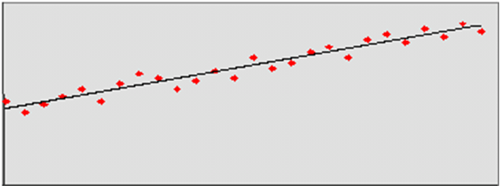
This method captures the trend of a series through the slope of the regression line while the series shifted by a cycle provides its seasonal profile. Using this method, the resulting forecast for the original series is calculated. The regression method provides a much better forecast of the series than was possible with the other exponential smoothing algorithms.
Based on the assumptions of the model that this method is trying to describe, versus the noisy data it is likely to receive, several exceptions to this regression technique are caught and corrected. First, since it is logically impossible to receive a negative value for the slope (such a value suggesting an inverse seasonality), whenever a negative slope is detected, the regression is rerun with the intercept fixed to zero. This guarantees that a positive slope is calculated and thus a more logical forecast is given.
The second noise-driven concession is to check the slope to determine if it is either too slight or too great. If this is the case, the method rejects itself out of hand and allows one of the other competing methods to provide the forecast.
The Profile-based forecasting method generates a forecast based on a seasonal profile. The profile may be loaded, manually entered, or generated by Curve. It can also be copied from another profile and adjusted.
The Profile-based forecasting method proceeds as follows:
The historical data and the profile are loaded.
The data is de-seasonalized using the profile and then fed to Simple method.
The alpha is capped by 0.5 by default or the Max Alpha (Profile) value entered by the user.
The Simple forecast is re-seasonalized using the profiles.
The Profile-based forecasting method can be successfully used to forecast new items. In order to do that, we need to have a profile (which can be copied from an item that shares the same seasonality) and a number that specifies the de-seasonalized demand (DD value). The forecast is calculated using the DD value multiplied by the profile. The confidence interval is set to 1/3 of the DD value.
If the DD value is used to forecast, the history (if it exists) of the product is ignored. Once we have enough history (number of data points exceed a global parameter), the forecast stops using the DD value, and it defaults to the normal Profile Based method.
|
Note: The Profile-based forecasting method is intended for a final forecasting level and not a source level. |
The Bayesian Forecasting method is based on combining historic sales data with sales plan data. It is especially effective for new products with little or no historic sales data.
Your sales plan can incorporate expert knowledge in two ways — shape and scale.
Shape is the selling profile or lifecycle that can be derived from a sales plan. For example, the shape for certain fashion items might show sales ramping up quickly for the first four weeks and then trailing off to nothing over the next eight weeks.
Scale, or magnitude, of a sales plan is the total quantity expected to be sold over the plan's duration.
Bayesian Forecasting assumes that the shape that sales takes is known, but the scale is uncertain. In Bayesian Forecasting, when no sales history is available, the sales forecast figures are equal to the sales plan figures. At this point, there is no reason to mistrust the sales plan. As point-of-sale data becomes available, the forecast is adjusted and the scale becomes a weighted average between the initial plan's scale and the scale reflected by known sales history. Confidence in the sales plan is controlled by the amount of sales data on hand and a Bayesian sensitivity constant (Bayesian Alpha), which you can set between zero and infinity.
Unlike standard time series forecasting, which requires only sales history to produce a forecast, Bayesian Forecasting requires a sales plan and sales history (if available). Because of this difference, Bayesian Forecasting is not included in AutoES. You must select it manually as a forecasting method in Forecast Administration or Forecast Maintenance.
Obtaining accurate short life-cycle product forecasts is very difficult, and standard statistical time series forecasting models frequently do not offer an adequate solution for many retailers. The following are major problems in automatically developing these forecasts:
The lack of substantial sales history for a product (which especially makes obtaining seasonal forecasts very difficult).
The difficulty of automatically matching a new product to a previous product or profile.
The inability to include planners' intuition into a forecasting model. For example, the overall sales level of the product, how quickly the product takes off, how the product's sales is affected by planned promotions.
Using a Bayesian approach, a short life-cycle forecasting algorithm was developed that begins with a product's seasonal sales plan (that is developed externally to the system by the planner).
As sales information arrives during the first few days or weeks of the season, the model generates a forecast by merging the information contained in the sales plan with the information contained in the initial sales data. These forecast updates can be critical to a company's success and can be used to increase or cancel vendor orders.
As forecasting consultants and software providers, Oracle Retail assists clients in obtaining good forecasts for future demands for their products based upon historical sales data and available causal information. Depending on the information available, Oracle Retail's software supports various forms of exponential smoothing and regression-based forecasting. Frequently, clients already have some expectations of future demands in the form of sales plans. Depending on the quality of their plans, they can provide very useful information to a forecasting algorithm (especially when only limited historical sales data is available). A forecasting algorithm was developed that merges a customer's sales plans with any available historical sales in a Bayesian fashion (that is, it uses new information to update or revise an existing set of probabilities.
In most retail situations, clients are interested in obtaining good product forecasts automatically with little or no human intervention. For stable products with years of historic sales data, our time series approaches (Simple, Holt, Winters, Regression based Causal, and so on) produce adequate results. The problem arises when attempting to forecast products with little or no history. In such instances, expert knowledge (generally in the form of sales plans) is required. Given that both sales plans and time series forecasts are available, an obvious question exists: When should the transition from sales plan to time series forecasting occur? In answering that question (in a particular scenario), suppose that we have determined that 13 weeks of history is the transition point. Does that mean that at 12 weeks the time series results are irrelevant and that at 14 weeks the sales plan has no value? Our intuition tells us that instead of a hard-edge boundary existing, there is actually a steady continuum where the benefits from the sales plan decrease as we gather more historic sales data. This was the motivation for developing an approach that would combine the two forecasts in a reasonable manner.
Bayesian forecasting is primarily designed for product/location positions for which a plan exists. These product/locations can be, but are not limited to: items new in the assortment, fashion items, and so on. The following guidelines should be followed:
No more than one plan should exist for a given product/location position. If multiple plans are to be set up for different time periods, the domain should be set up with different forecasting levels for each time period of interest.
Any time period with non-zero Actuals for a given product/location position should have a corresponding plan component. Otherwise, the system assumes a plan exists and equals zero and acts accordingly.
The time period of interest for the Bayesian algorithm starts with the first non-zero value of the plan or the history start date (whichever is more recent), and ends at the end of the forecast horizon.
LoadPlan Forecasting Method copies the measure that was specified as Data Plan in the Forecast Administration Workbook into the Forecast measure. This method does not generate confidence and cumulative intervals when it is the final level method and no source level is specified. This method only generates confidence and cumulative intervals when a source level is specified and the source and final levels are the same.
Copy Forecasting Method copies the measure that was specified as Forecast Data Source in the Forecast Administration Workbook into the Forecast measure. This method does not generate confidence and cumulative intervals.
Causal, or promotional, forecasting requires four input streams:
Time Series Data
Historical Promotional Calendar
Baseline Forecasts
Future Promotional Calendar
Promote decomposes the problem of promotional forecasting into two sub-tasks:
Estimating the effect that promotions have on demand
Applying the effects on the baseline forecasts
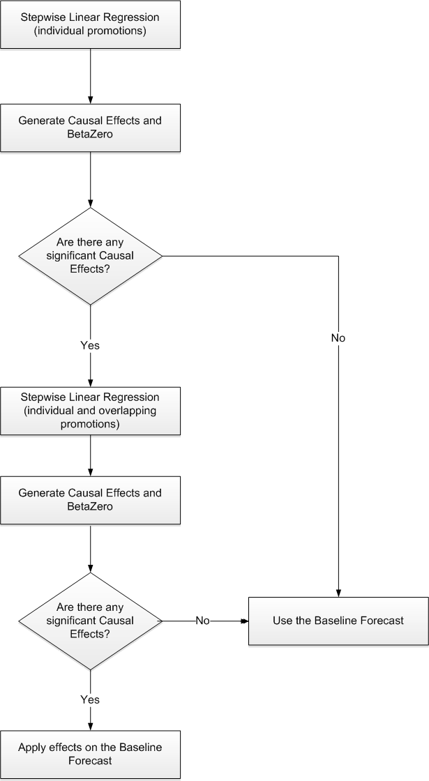
To accomplish the first task, a stepwise regression sub-routine is used. This routine takes a time series and a collection of promotional variables and determines which variables are most relevant and what effect those relevant variables have on the series.
A promotion variable can represent an individual promotion or a combination of overlapping promotions. An individual promotion represents the case where for a particular time period a single promotion is enabled. Overlapping promotions represents the case where there are two or more promotions that happen at the same time period at the same location for the same product. Causal Forecasting Method can calculate not only each individual promotion effect, but also the overlapping promotions effects.
Thus, the output from the algorithm is a selection of promotional variables and the effects of those variables on the series. In the second step, knowing the effects and the baseline forecasts, we can generate a promotional forecast by applying the effects wherever the promotion or the overlapping promotion are active in the future.
The causal forecasting process has been simplified by first estimating the effects of promotions. Then the effects are applied on top of a baseline that is created externally from the causal forecasting process. For example, the baseline can be a loaded measure, or it can be generated in RDF using AutoES and source-level techniques.
It should be noted that just because promotional forecasting is selected, it does not necessarily imply that a promotional forecast results. In some instances, no promotional variables are found to be statistically significant. In these cases, the forecast ends up equivalent to standard time series forecasts.
If you want to force certain promotional variables into the model, this can be managed through forecasting maintenance parameters.
The Oracle Retail experience in promotional forecasting has led us to believe that there are a few requirements that are necessary to successfully forecast retail promotions:
Baseline forecasts need to consider seasonality; otherwise normal seasonal demand is attributed to promotional effects.
Promotional Effects need to be able to be analyzed at higher levels in the retail product and location hierarchies. This produces cleaner signals and alleviates issues involved in forecasting new items and new stores and issues involving data sparsity.
Users need to be aware that the forecasting models cannot tell the difference between causal effects and correlated effects. What this means is that users should be wary of promotional effects attributed to an event that occurs at the same time every year. The system cannot distinguish between the promotional effect and the normal seasonality of the product. The same can be said for any two events that always occur at the same time. The combined effect is most likely attributed to one or the other event.
Rather than use a sales history that may not have sufficient or accurate data, users can load a baseline into the RDF Causal Engine instead. Baselines are often generated using data that is rolled up to a higher dimension than item/store, providing a greater depth of data and hence a less-noisy sales history. The sales data used to generate the baseline can be corrected for out-of-stock, promotional, and other short-term event information using Preprocessing. These baselines are then spread back to the item/store level and then loaded in the RDF Causal Engine. The Engine uses the baseline along with the historic promotional data and future planned promotions data to create the system forecast, which is the baseline with the lifts, which were calculated from the promotional data, applied on top.
When a baseline is used, the AutoES binary code executes in the following manner:
The binary reads the history of the time series.
The binary reads the type of each promotional variable into the system.
The binary reads in all the promotional variables that apply to the series.
The binary creates an internal promotional variable to allow the modeling of trend.
Promotional variables, internal promotional variables, promotional variable types, and the series itself are passed to the stepwise regression routine, with the historic data serving as the dependent variables.
If the regression finds no significant promotional variables, the casual method is considered to have failed to fit. In this case, the forecast equals the baseline.
The fit at time t, fit(t), is defined in terms of bo, the intercept of the regression, b1, the effect corresponding to promotional variable i, and pi(t), is the value of promo variable I, in time t as:
fit(t) = bo + å bo*pi(t)
The forecast is obtained by re-causalizing the baseline. This is done by adding back the causal effects for the product/location/time positions, where the corresponding promo variables are on in the forecast region.
The binary writes the winning promotional variables effects back to the database.
The selected model is recorded in the database.
The binary records the forecast and the baseline in the database.
To forecast short-lifecycle promotional items, Causal deprices, depromotes, and smoothes the forecasting data source to generate the short lifecycle forecast causal baseline. In essence, this is the causal forecasting process where the generation of the baseline and the estimation of the promotional lifts are modified for items with short lifecycle.
First, the baseline is generated. Then the forecast data source is depriced, depromoted and smoothed. The resulting feed is aggregated and then spread down using rate of sales as a profile to create a lifecycle curve. The lifecycle curve is shifted and stretched or shrunk to fit the new season length. This curve represents the pre-season baseline forecast. In season, the pre-season forecast serves as a forecast plan to the Bayesian forecasting method. The Bayesian forecast is the causal baseline for short lifecycle items.The next step is to calculate the promotional lifts.
To do this, the promotional lifts are filtered from the historical sales and applied on top of the item's rate of sale. The resulting measure is regressed against the promotional variables to determine the promotion effects. Finally, the promotion effects are applied on top of the short-lifecycle causal baseline to generate the final forecast.
The causal forecasting at the daily level is calculated by spreading the weekly causal forecast down to day. The spreading utilizes causal daily profiles, thus obtaining a causal forecast at the day granularity.
The daily casual forecast process executes in the following manner:
Preprocess the day-level promotional variables by multiplication with daily profiles. Aggregate the preprocessed continuous day level promotional variables to the week level.
Calculate the causal forecast at the weekly level. Set promotional effects if desired. Use the RDF causal engine to generate the forecast.
Calculate the multiplicative promotional effects at the item/store level for every promo variable. The effects can be either:
Manually preset (See Step 1).
Calculated. When calculating the causal forecast, the calculated causal effects are written back to the database. If the effects are calculated at higher level than item/store, the effects are replicated down to item/store since the effects are multiplicative. If source-level forecasting is used and causal method is used both at the source-level and at the final-level, the effects from the final-level is used.
Daily profiles are calculated using the Curve module. Since as much history as possible is used and is averaged over seven days, it's assumed that these profiles are de-causalized. The de-causalized daily profiles capture the day-of-week effect and should be quite stable.
Causal effects are applied to the daily profiles. The profiles are multiplied by the causal effects and then the profiles have to renormalize.
For every item/store combination, calculate a normal week-to-day profile based on historic data. Note that this profile is already computed for spreading the weekly forecasts to the day level. Suppose for a certain product, the profile is as follows:
| Mon | Tues | Wed | Thu | Fri | Sat | Sun | Week |
|---|---|---|---|---|---|---|---|
| 10% | 10% | 10% | 10% | 20% | 30% | 10% | 100% |
Suppose that in the past, the promotion was held on Wednesday, Thursday, and Friday of week w6:
| Mon | Tues | Wed | Thu | Fri | Sat | Sun |
|---|---|---|---|---|---|---|
| P | P | P |
Then the continuous weekly indicator for this promotion in w6 should be set to 0.4, which is the sum of the weights of Wednesday, Thursday, and Friday.
Now assume that the same promotion is held in a future week (w36), but only on Thursday:
| Mon | Tues | Wed | Thu | Fri | Sat | Sun |
|---|---|---|---|---|---|---|
| P |
Then the continuous weekly indicator for w36 should be set to 0.1, which is the weight of Thursday only.
The approach to use the continuous promotion indicators to generate an accurate causal forecast at the day level is as follows:
Calculate the weekly multiplicative effect for the promotion using the standard causal forecasting system with continuous indicators.
Calculate the forecast for w36 using the standard causal forecasting system with continuous indicators.
Update the week-to-day profile of w36 so that the weight of Thursday is doubled (the multiplicative factor is 2):
| Mon | Tues | Wed | Thu | Fri | Sat | Sun | Week |
|---|---|---|---|---|---|---|---|
| 10% | 10% | 10% | 20% | 20% | 30% | 10% | 110% |
Normalize the profile for w36:
| Mon | Tues | Wed | Thu | Fri | Sat | Sun | Week |
|---|---|---|---|---|---|---|---|
| 9% | 9% | 9% | 18% | 18% | 27% | 9% | 100% |
Finally, spread the forecast of w36 using the normalized profile.
In the Oracle Retail approach to causal forecasting, the causal effects are obtained by fitting a stepwise linear regression model that determines which variables are most relevant and what effect those relevant variables have on the series. The data used to fit the regression is the fit history of each time series, so basically a model is fit per time series. A problem arises due to potential lack of significant data (that is, when a promotional variable is not represented in the history, but it is present in the forecast region). In that case, the effect for that variable would not be computed at all, thus affecting the accuracy of the forecast. There are a few solutions that make use of the effects from other similar time series. One solution would be to do source-level causal forecasting and then spread down to the final-level.
This would be equivalent to using the effects at the source-level for time series that have no causal variable instances in the history. This has a serious conceptual drawback. By aggregating the promotional variables at the source-level, we would force the effects on the other time series in the same aggregation class that would otherwise not have the causal variables on at the same time. An alternate solution is whenever a causal effect cannot be computed because of lack of significant data. An averaged effect from another time-series in the same aggregation class is going to be used instead. Refer to Table 13-3, "Promo Effect Types" for information on the Override Higher Level type.